Production Surveillance
Description
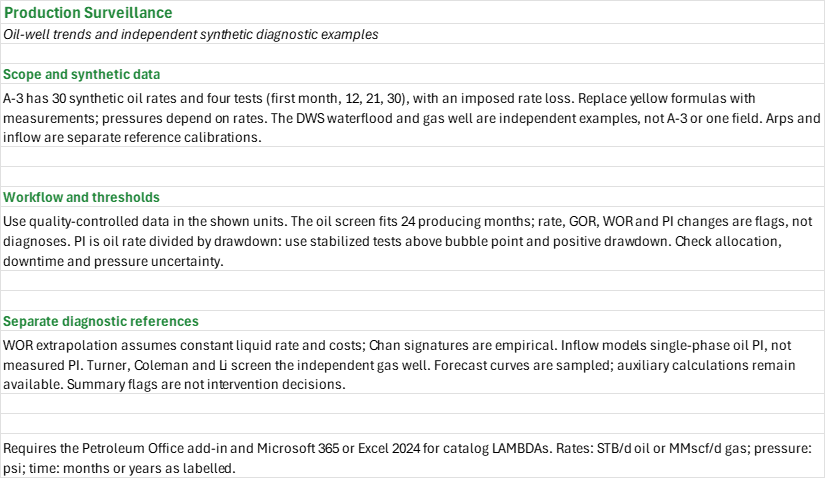
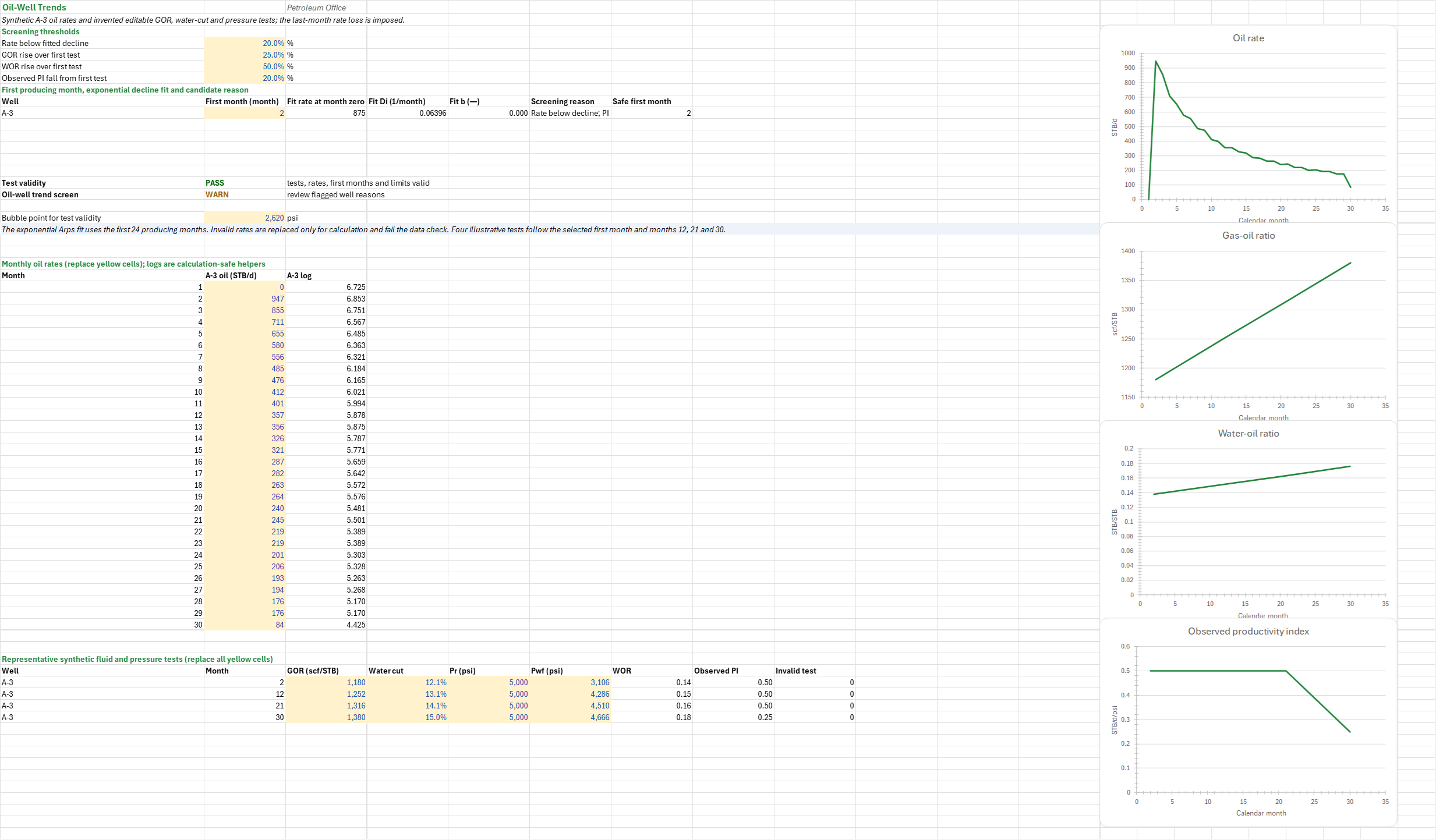
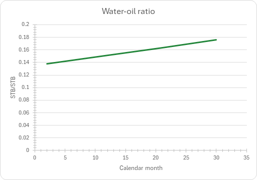
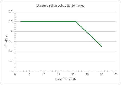
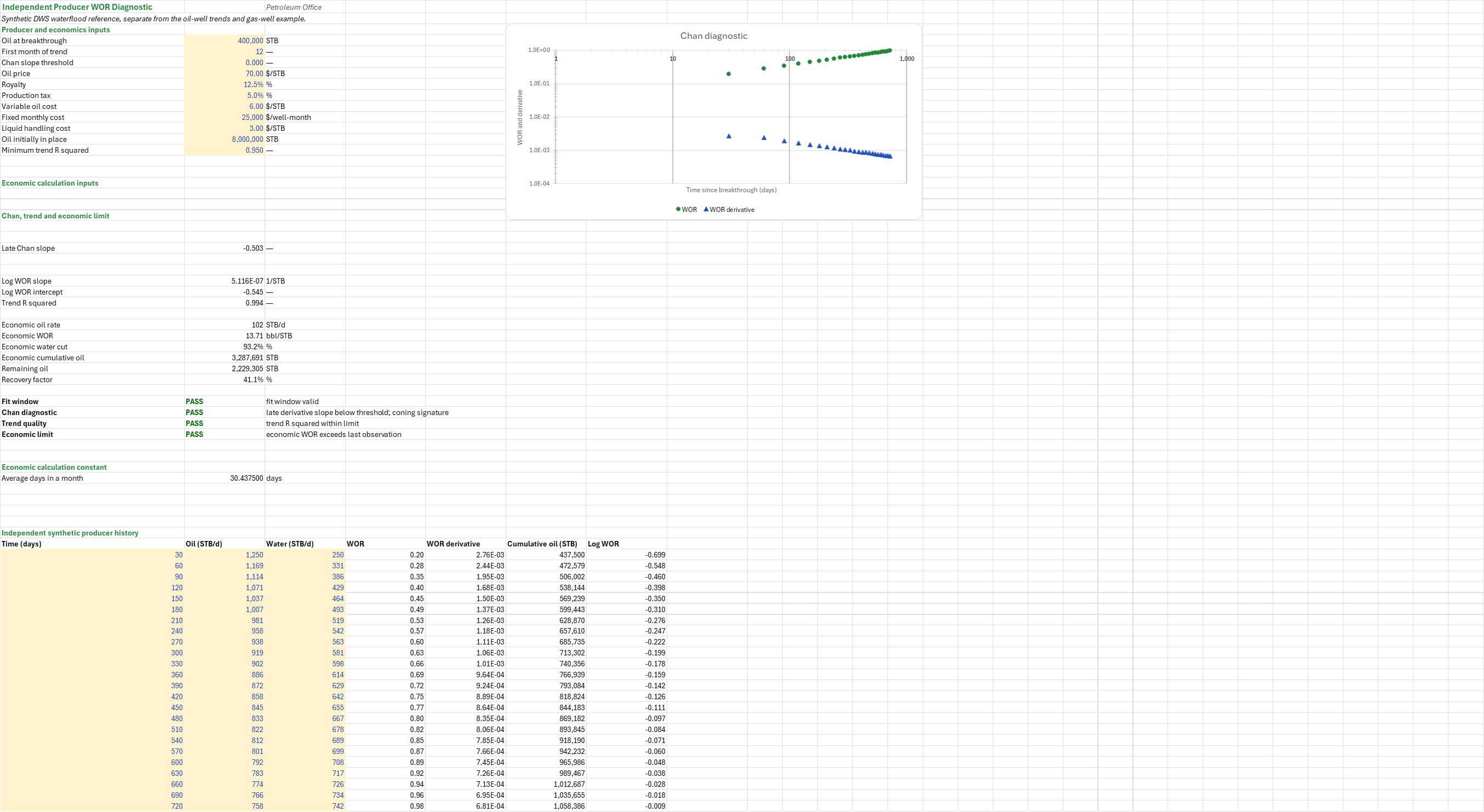
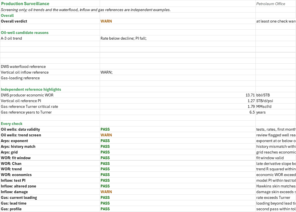
Has this oil well's rate fallen below its decline, or its gas-oil ratio (GOR), water-oil ratio (WOR) or observed productivity index (PI) moved enough to look into? You enter monthly oil rates, four well tests and your screening limits. You read off an exponential decline fit, each trend against its limit and the candidate reason, beside four independent references: an Arps forecast, a waterflood producer's WOR, vertical oil inflow and gas-well loading. These synthetic examples are not a matched field.
How to use it: Replace the yellow inputs and synthetic observations with consistent measurements. On the Well trends sheet, calculate oil rate from produced volume and producing days, checking allocation and downtime; enter the true first producing month (1–7 in this layout), all required rates, and the four tests' GOR, water cut and reservoir and flowing pressures. Invalid tests or first months fail the data check; calculation-safe substitute rates are not results. For PI, use representative reservoir and stabilized flowing pressures above the bubble point with positive drawdown. Each reference sheet has its own inputs; changing one does not change the others. Gas loading is not inferred from the oil well's GOR. The Summary combines the candidate reasons and every check for review, not automatic intervention.
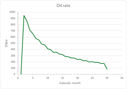
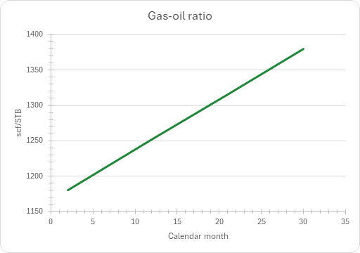
Method: Well trends uses A-3's 30 synthetic type-well oil rates and month-30 GOR and water cut. The tests at the selected first month and months 12, 21 and 30, the fluid trajectories, the pressures and the imposed month-30 rate loss are invented; yellow rate and test formulas are editable, and pressures depend on rates. A log-rate fit to the first 24 producing months gives an exponential Arps baseline (b = 0) with nonnegative decline. The latest rate is compared with the fit, and GOR, WOR and observed PI with the first test. WOR = water cut / (1 - water cut); PI = oil rate / pressure drawdown. Thresholds are screening choices, not diagnostic limits.
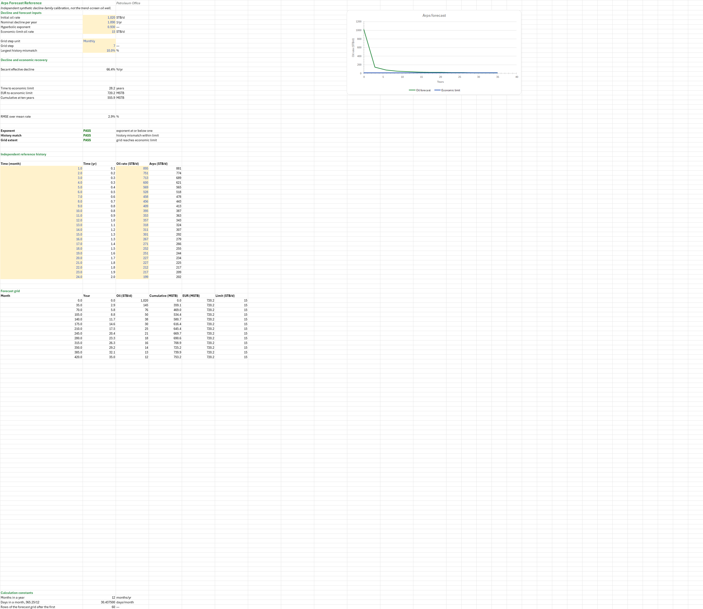
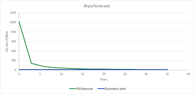
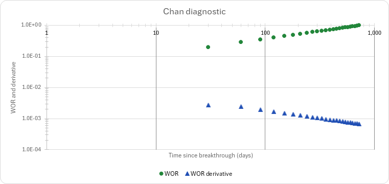
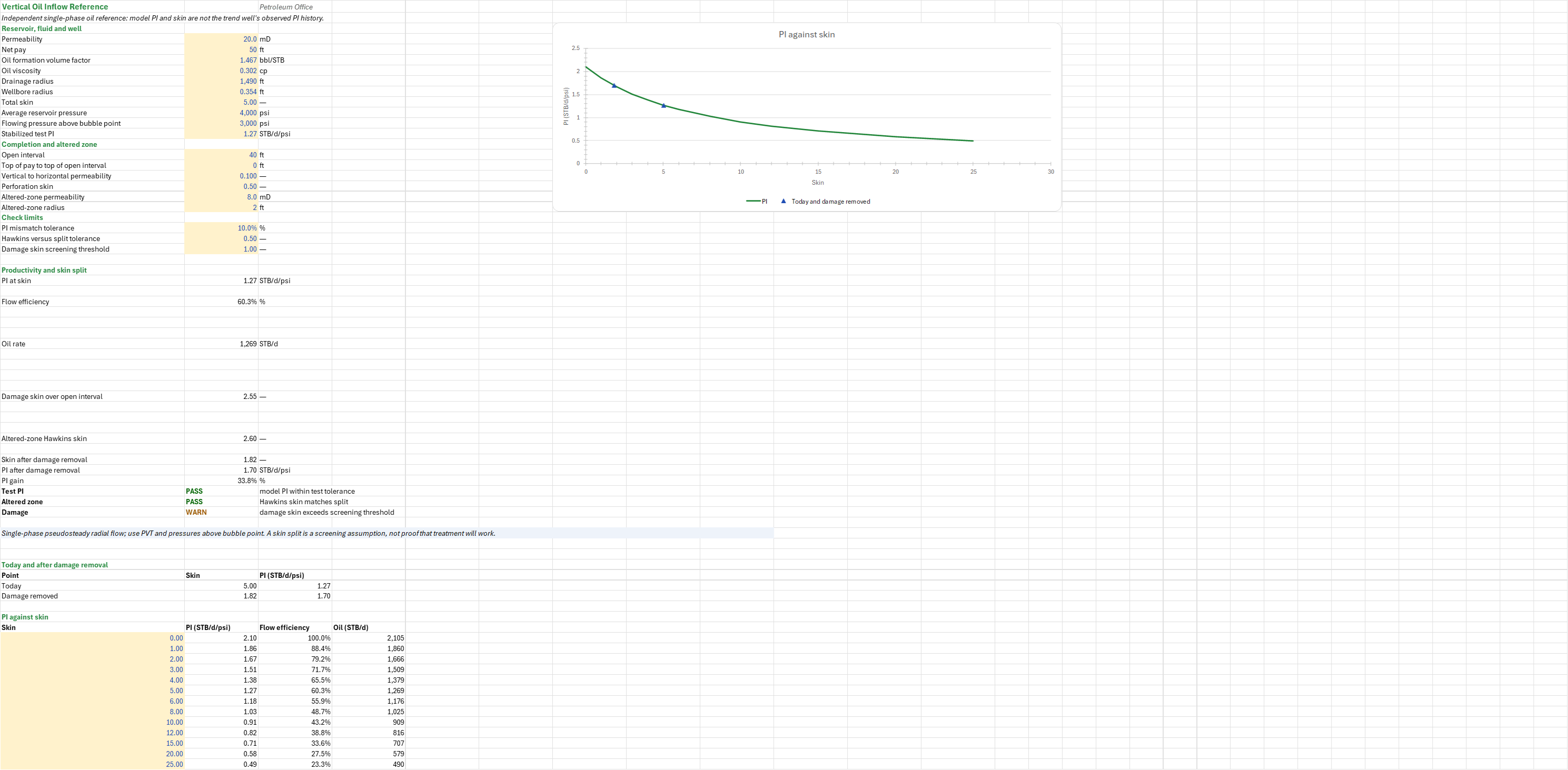
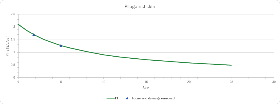
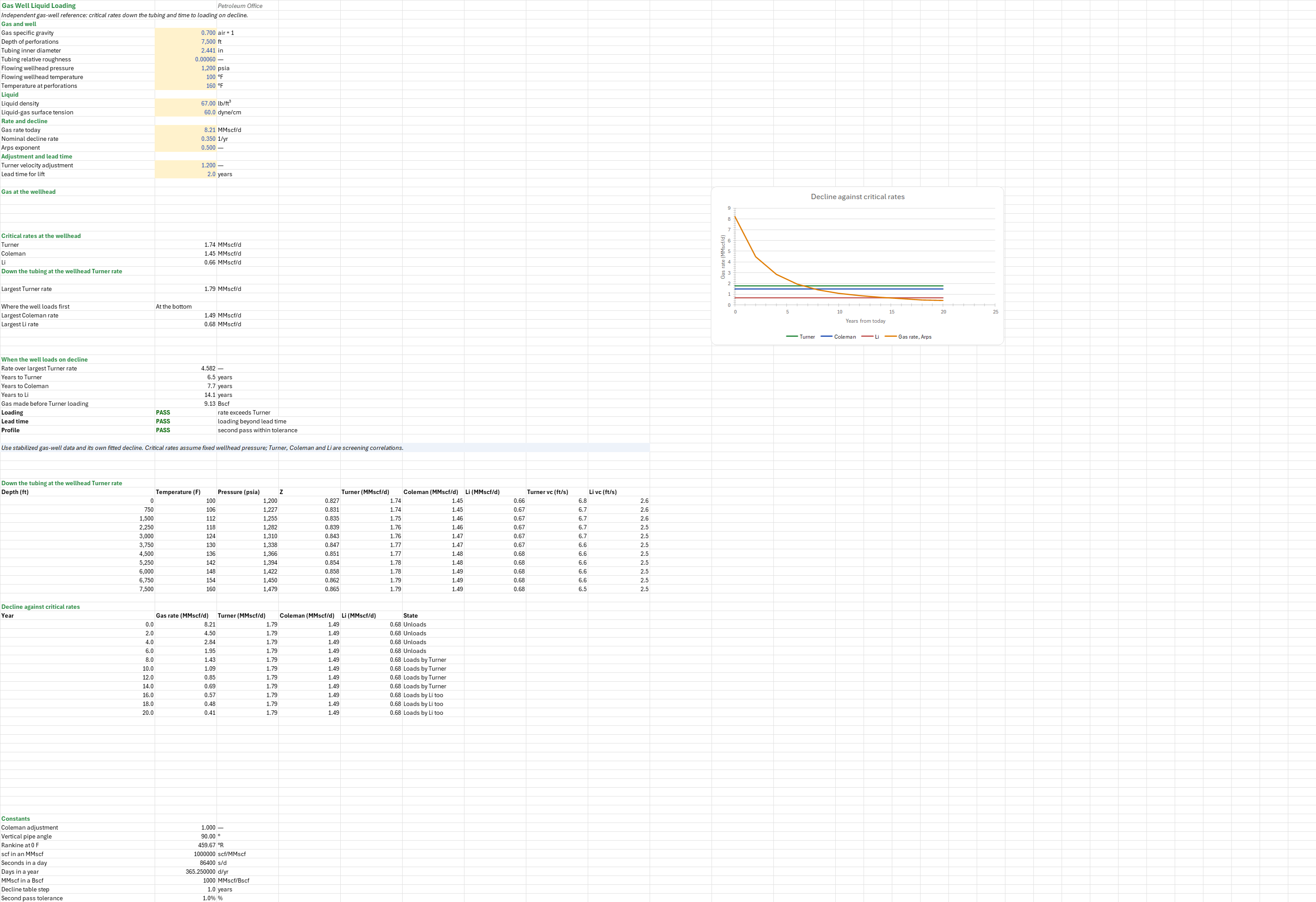
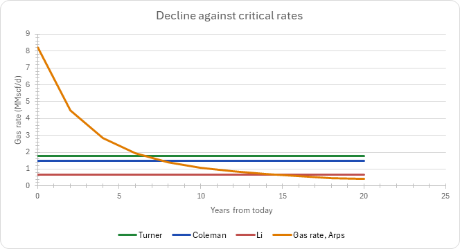
The Arps reference is an independent decline example. The DWS waterflood reference uses Chan's derivative and extrapolates log WOR to an economic limit at constant liquid rate and costs. The separate single-phase inflow model computes PI, the skin split and the potential gain on damage removal, not A-3's observed PI. The independent gas example compares Turner, Coleman and Li critical rates along the tubing and against gas decline.
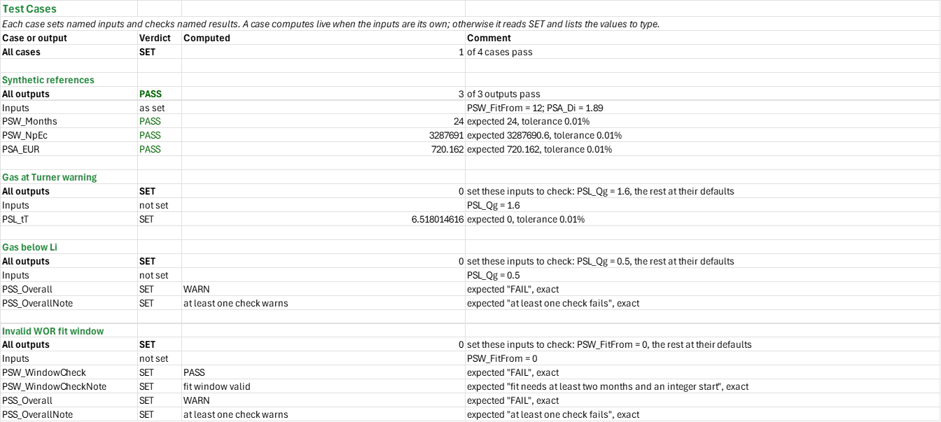
Example: With the independent reference defaults (the WOR trend from month 12 and the Arps reference's nominal decline of 1.89 per year), the 24-month WOR history gives an economic cumulative oil of approximately 3,287,690.6 STB, while the separate Arps reference gives an EUR of approximately 720.162 MSTB. These are synthetic reference results, not a forecast for A-3.
Validity
Illustrative pressures exceed the 2620 psi bubble point; test conditions and pressure uncertainty can mimic a PI trend. The exponential fit screens, it does not forecast reserves; fit representative production and investigate outliers. A rate, GOR, WOR or PI flag does not prove a cause. Chan signatures are empirical and WOR extrapolation may not persist. Inflow assumes single-phase pseudosteady radial flow; skin decomposition does not prove treatment response. Loading assumes the entered water properties, fixed wellhead pressure and Arps decline; confirm with a stabilized gas test and flowing gradient. Review uncertainty and economics before action.
References
- Arps, J.J. (1945). Analysis of Decline Curves. Transactions of the AIME, 160, 228-247.
- Chan, K.S. (1995). Water Control Diagnostic Plots. SPE 30775.
- Turner, R.G., Hubbard, M.G. and Dukler, A.E. (1969). Analysis and Prediction of Minimum Flow Rate for the Continuous Removal of Liquids from Gas Wells. SPE 2198.
Inputs
| Input | Unit | Default | Name |
|---|---|---|---|
| First month (Well trends fit table) | month | 2 | PSH_Start1 |
| Rate below fitted decline, GOR rise over first test, WOR rise over first test, observed PI fall from first test | fraction | 0.20, 0.25, 0.50, 0.20 | PSH_RateDrop, PSH_GorRise, PSH_WorRise, PSH_PiDrop |
| Bubble point for test validity | psi | 2620 | PSH_Pb |
| Initial oil rate, nominal decline per year, hyperbolic exponent, economic-limit oil rate (Arps reference) | STB/d, 1/year, fraction, STB/d | 1020, 1.89, 0.93, 15 | PSA_qi, PSA_Di, PSA_b, PSA_QEcon |
| Grid step unit, grid step, largest history mismatch | text, months or days, fraction | Monthly, 7, 0.1 | PSA_Basis, PSA_Step, PSA_FitMax |
| Oil at breakthrough, first month of trend, Chan slope threshold | STB, month, fraction | 400000, 12, 0 | PSW_Np0, PSW_FitFrom, PSW_SlopeConing |
| Oil price, royalty, production tax, variable oil cost, fixed monthly cost, liquid handling cost | $/STB, fraction, fraction, $/STB, $/month, $/STB | 70, 0.125, 0.05, 6, 25000, 3 | PSW_Price, PSW_Royalty, PSW_Tax, PSW_Opex, PSW_Fixed, PSW_Lift |
| Oil initially in place, minimum trend R squared | STB, fraction | 8000000, 0.95 | PSW_N, PSW_R2Min |
| Permeability, net pay, oil formation volume factor, oil viscosity, drainage radius, wellbore radius, total skin | mD, ft, rb/STB, cP, ft, ft, fraction | 20, 50, 1.467, 0.302, 1490, 0.354, 5 | PSI_k, PSI_h, PSI_Bo, PSI_Uo, PSI_re, PSI_rw, PSI_s |
| Average reservoir pressure, flowing pressure above bubble point, stabilized test PI | psi, psi, STB/d/psi | 4000, 3000, 1.27 | PSI_Pr, PSI_Pwf, PSI_JTest |
| Open interval, top of pay to top of open interval, vertical to horizontal permeability, perforation skin | ft, ft, fraction, skin | 40, 0, 0.1, 0.5 | PSI_hp, PSI_htop, PSI_kvkh, PSI_sp |
| Altered-zone permeability and radius | mD, ft | 8, 2 | PSI_ks, PSI_rs |
| PI mismatch tolerance, Hawkins versus split tolerance, damage skin screening threshold | fraction, skin, skin | 0.1, 0.5, 1 | PSI_JTol, PSI_sTol, PSI_sdMax |
| Gas specific gravity, depth of perforations, tubing inner diameter, tubing relative roughness | fraction, ft, in, fraction | 0.7, 7500, 2.441, 0.0006 | PSL_SGg, PSL_TVD, PSL_ID, PSL_Rough |
| Flowing wellhead pressure, flowing wellhead temperature, temperature at perforations | psia, F, F | 1200, 100, 160 | PSL_Pwh, PSL_Twh, PSL_Tbh |
| Liquid density, liquid-gas surface tension | lb/ft3, dyne/cm | 67, 60 | PSL_RhoL, PSL_IFT |
| Gas rate today, nominal decline rate, Arps exponent | MMscf/d, 1/year, fraction | 8.21, 0.35, 0.5 | PSL_Qg, PSL_Di, PSL_b |
| Turner velocity adjustment, lead time for lift | fraction, years | 1.2, 2 | PSL_TurnerF, PSL_Lead |
Editable tables: Well trends B25:B54 contains 30 monthly oil rates, and C59:F62 contains four GOR, water-cut, reservoir-pressure and flowing-pressure tests. The Arps reference A36:A59 and C36:C59 contain 24 history times and oil rates. WOR diagnostics A51:C74 contains 24 independent time, oil and water observations. Inflow reference A61:A73 contains the skin sweep. Each reference has its own inputs; changing one does not change the others.
Sheets
Guide— synthetic scope, workflow and interpretation.Well trends— one oil well's rate, GOR, WOR and observed-PI histories, the exponential decline fit and the candidate reason.Arps reference— an independent calibrated Arps decline history and forecast to the economic limit.WOR diagnostics— an independent DWS waterflood producer's Chan derivative and its WOR extrapolated to an economic limit.Inflow reference— an independent vertical oil well's PI, skin split and skin sensitivity.Gas loading— an independent gas well's tubing profile, Turner, Coleman and Li critical rates, and decline.Summary— candidate reasons, reference highlights and every named check; a fail overrides a warning.Test Cases— the worked example and other cases, with expected and computed results.
Functions used
Names (182)
| Name | Refers to | Comment |
|---|---|---|
PO.CO.Damage.DecompositionLAMBDA |
=LAMBDA(s_t, s_p, h, h_p, h_top, r_w, kv_kh, IF((h<=0)+(h_p<=0)+(h_p>h)+(h_top<0)+(h_top+h_p>h)+(r_w<=0)+(kv_kh<=0), NA(), LET(hp_d, h_p/h, ht_d, h_top/h, r_d, r_w/h*SQRT(kv_kh), a_term, 1/(ht_d+hp_d/4), b_term, 1/(ht_d+3*hp_d/4), s_c, (1/hp_d-1)*LN(PI()/(2*r_d))+1/hp_d*LN(hp_d/(2+hp_d)*SQRT((a_term-1)/(b_term-1))), hp_d*(s_t-s_c)-s_p))) |
Damage skin s_d left in a test's total skin s_t: (h_p/h)*(s_t - s_c) - s_p (Saidikowski), s_c the Papatzacos partial-penetration skin of h_p ft open h_top ft below the top of h ft of pay, s_p the perforation skin. |
PO.CO.Damage.FlowLAMBDA |
=LAMBDA(j_actual, j_ideal, measure, IF((j_actual<=0)+(j_ideal<=0), NA(), IF(measure="FE", j_actual/j_ideal, IF(measure="DR", j_ideal/j_actual, IF(measure="DF", 1-j_actual/j_ideal, NA()))))) |
Flow efficiency of a well from its PI j_actual and its undamaged PI j_ideal: measure "FE" gives j_actual/j_ideal, "DR" the damage ratio j_ideal/j_actual, "DF" the damage factor 1 - j_actual/j_ideal. |
PO.CO.Damage.HawkinsLAMBDA |
=LAMBDA(k, k_s, r_s, r_w, IF((k<=0)+(k_s<=0)+(r_w<=0)+(r_s<r_w), NA(), (k/k_s-1)*LN(r_s/r_w))) |
Hawkins (1956) skin of an altered zone round the wellbore: (k/k_s - 1)*ln(r_s/r_w). k formation and k_s altered-zone permeability (mD), r_s altered-zone and r_w wellbore radius (ft). Positive when damaged, negative when stimulated. |
PO.DCA.Arps.SecantEffLAMBDA |
=LAMBDA(Di, b, IF(OR(Di<0, b<0), NA(), IF(b=0, 1-EXP(-Di), 1-(1+b*Di)^(-1/b)))) |
Secant effective decline (fraction per period) of an Arps hyperbolic: 1 - (1 + b*Di)^(-1/b), or 1 - exp(-Di) for b = 0. Di is the nominal decline per period (1/yr gives the effective annual decline) and b the exponent. |
PO.PE.Chan.WORDerivativeLAMBDA |
=LAMBDA(time, wor, at, LET(n, COUNT(time), k, MATCH(at, time, 0), k_lo, MAX(1, k-1), k_hi, MIN(n, k+1), t_k, INDEX(time, k), t_lo, INDEX(time, k_lo), t_hi, INDEX(time, k_hi), w_k, INDEX(wor, k), w_lo, INDEX(wor, k_lo), w_hi, INDEX(wor, k_hi), IF(k=1, (w_hi-w_k)/(t_hi-t_k), IF(k=n, (w_k-w_lo)/(t_k-t_lo), ((w_k-w_lo)/(t_k-t_lo)*(t_hi-t_k)+(w_hi-w_k)/(t_hi-t_k)*(t_k-t_lo))/(t_hi-t_lo))))) |
Chan (1995) WOR′: the time derivative of the water-oil ratio at one point of a production history, a three-point difference weighted by the neighbouring intervals, [1/time unit]. |
PO.PE.Loading.LiRateLAMBDA |
=LAMBDA(p_psia, t_degF, sg_gas, tubingID_in, sigma_dyncm, rhoL_lbft3, IF(OR(p_psia<=0, t_degF<=-459.67, sg_gas<=0, tubingID_in<=0, sigma_dyncm<=0, rhoL_lbft3<=0), NA(), LET(tr, t_degF+459.67, z, PO.PVT.Z.ByDAK(p_psia/PO.PVT.Ppc.BySutton(sg_gas), tr/PO.PVT.Tpc.BySutton(sg_gas)), rho_g, PO.PVT.Rho.Gas.ByDefinition(p_psia, tr, sg_gas, z)*62.428, IF(rhoL_lbft3<=rho_g, NA(), 3.06*p_psia*0.72907*sigma_dyncm^0.25*(rhoL_lbft3-rho_g)^0.25/rho_g^0.5*PI()*tubingID_in^2/576/(tr*z))))) |
Li critical gas rate to unload liquid (flat-droplet model), MMscf/d: p_psia and t_degF where it is read, gas gravity sg_gas, tubingID_in, the liquid's sigma_dyncm and rhoL_lbft3. Same order as PO.PE.Loading.TurnerRate. |
PO.PE.Loading.TurnerRateLAMBDA |
=LAMBDA(p, t, sg_g, tubing_id, sigma, rho_l, factor, IF(OR(p<=0, t<=-459.67, sg_g<=0, tubing_id<=0, sigma<=0, rho_l<=0, factor<=0), NA(), LET(tr, t+459.67, z, PO.PVT.Z.ByDAK(p/PO.PVT.Ppc.BySutton(sg_g), tr/PO.PVT.Tpc.BySutton(sg_g)), rho_g, PO.PVT.Rho.Gas.ByDefinition(p, tr, sg_g, z)*62.428, IF(rho_l<=rho_g, NA(), 3.06*p*factor*1.593*sigma^0.25*(rho_l-rho_g)^0.25/rho_g^0.5*PI()*tubing_id^2/576/(tr*z))))) |
Turner critical gas rate to unload liquid, MMscf/d: p (psia) and t (°F) where it is read, usually the wellhead, gas gravity sg_g, tubing_id (in), the liquid's sigma (dyne/cm) and rho_l (lb/ft³), and factor (1.2 Turner, 1 Coleman). |
PO.RES.Reserves.EconLimitLAMBDA |
=LAMBDA(Price, Royalty, Tax, Opex, Fixed, LET(netback, Price*(1-Royalty)*(1-Tax)-Opex, IF(netback>0, Fixed/netback, NA()))) |
Economic-limit rate: fixed cost per period over the netback per unit after royalty, production tax and variable opex; #N/A if the netback is not positive |
PSA_BCheck |
'Arps reference'!$B$28 |
Exponent verdict |
PSA_BCheckNote |
'Arps reference'!$C$28 |
Exponent comment |
PSA_Basis |
'Arps reference'!$B$9 |
Grid step unit |
PSA_DMo |
'Arps reference'!$B$128 |
Days in a month, 365.25/12, days/month |
PSA_DeSec |
'Arps reference'!$B$15 |
Secant effective decline, %/yr |
PSA_Di |
'Arps reference'!$B$5 |
Nominal decline per year, 1/yr |
PSA_EUR |
'Arps reference'!$B$20 |
EUR to economic limit, MSTB |
PSA_FitCheck |
'Arps reference'!$B$29 |
History match verdict |
PSA_FitCheckNote |
'Arps reference'!$C$29 |
History match comment |
PSA_FitMax |
'Arps reference'!$B$11 |
Largest history mismatch, % |
PSA_Forecast |
'Arps reference'!$A$64:$F$76 |
Month, Year, Oil (STB/d), Cumulative (MSTB), EUR (MSTB), Limit (STB/d) |
PSA_GridCheck |
'Arps reference'!$B$30 |
Grid extent verdict |
PSA_GridCheckNote |
'Arps reference'!$C$30 |
Grid extent comment |
PSA_HistQ |
'Arps reference'!$C$36:$C$59 |
History oil rates, STB/d |
PSA_HistT |
'Arps reference'!$A$36:$A$59 |
History times, months |
PSA_History |
'Arps reference'!$A$36:$D$59 |
Time (month), Time (yr), Oil rate (STB/d), Arps (STB/d) |
PSA_Inputs |
'Arps reference'!$B$4:$B$11 |
Arps parameters, economic limit, grid and fit tolerance |
PSA_MoYr |
'Arps reference'!$B$127 |
Months in a year, months/yr |
PSA_Np10 |
'Arps reference'!$B$21 |
Cumulative at ten years, MSTB |
PSA_QEcon |
'Arps reference'!$B$7 |
Economic-limit oil rate, STB/d |
PSA_RelErr |
'Arps reference'!$B$25 |
RMSE over mean rate, % |
PSA_Results |
'Arps reference'!$B$14:$B$30 |
Decline, economic limit, history fit and checks |
PSA_Rows |
'Arps reference'!$B$129 |
Rows of the forecast grid after the first |
PSA_Step |
'Arps reference'!$B$10 |
Grid step |
PSA_TLim |
'Arps reference'!$B$19 |
Time to economic limit, years |
PSA_b |
'Arps reference'!$B$6 |
Hyperbolic exponent |
PSA_qi |
'Arps reference'!$B$4 |
Initial oil rate, STB/d |
PSH_DataCheck |
'Well trends'!$B$16 |
Test validity verdict |
PSH_DataCheckNote |
'Well trends'!$C$16 |
Test validity comment |
PSH_Di1 |
'Well trends'!$D$10 |
Exponential monthly decline |
PSH_Fits |
'Well trends'!$A$10:$G$10 |
Well, First month (month), Fit rate at month zero (STB/d), Fit Di (1/month), Fit b (—), Screening reason, Safe first month |
PSH_GorRise |
'Well trends'!$B$5 |
GOR rise over first test, % |
PSH_Inputs |
'Well trends'!$B$4:$B$7 |
Selected screening thresholds, not diagnostic limits |
PSH_Pb |
'Well trends'!$B$19 |
Bubble point for test validity, psi |
PSH_PiDrop |
'Well trends'!$B$7 |
Observed PI fall from first test, % |
PSH_QNow1 |
'Well trends'!$B$54 |
Last oil rate, STB/d |
PSH_Qi1 |
'Well trends'!$C$10 |
Rate at month zero from exponential fit |
PSH_RateDrop |
'Well trends'!$B$4 |
Rate below fitted decline, % |
PSH_Rates |
'Well trends'!$A$25:$C$54 |
Month, A-3 oil (STB/d), A-3 log |
PSH_Reason1 |
'Well trends'!$F$10 |
Candidate reason |
PSH_Start1 |
'Well trends'!$B$10 |
First producing calendar month |
PSH_Tests |
'Well trends'!$A$59:$I$62 |
Well, Month, GOR (scf/STB), Water cut, Pr (psi), Pwf (psi), WOR, Observed PI, Invalid test |
PSH_TrendCheck |
'Well trends'!$B$17 |
Oil-well trend screen verdict |
PSH_TrendCheckNote |
'Well trends'!$C$17 |
Oil-well trend screen comment |
PSH_WorRise |
'Well trends'!$B$6 |
WOR rise over first test, % |
PSH_b1 |
'Well trends'!$E$10 |
Exponential Arps exponent |
PSI_Bo |
'Inflow reference'!$B$6 |
Oil formation volume factor, bbl/STB |
PSI_DamCheck |
'Inflow reference'!$B$49 |
Damage verdict |
PSI_DamCheckNote |
'Inflow reference'!$C$49 |
Damage comment |
PSI_FE |
'Inflow reference'!$B$29 |
Flow efficiency, % |
PSI_Gain |
'Inflow reference'!$B$46 |
PI gain, % |
PSI_Inputs |
'Inflow reference'!$B$4:$B$24 |
Independent reservoir, fluid, well, completion and check inputs |
PSI_J |
'Inflow reference'!$B$27 |
PI at skin, STB/d/psi |
PSI_JCheck |
'Inflow reference'!$B$47 |
Test PI verdict |
PSI_JCheckNote |
'Inflow reference'!$C$47 |
Test PI comment |
PSI_JTest |
'Inflow reference'!$B$13 |
Stabilized test PI, STB/d/psi |
PSI_JTol |
'Inflow reference'!$B$22 |
PI mismatch tolerance, % |
PSI_JTreat |
'Inflow reference'!$B$45 |
PI after damage removal, STB/d/psi |
PSI_Points |
'Inflow reference'!$A$56:$C$57 |
Point, Skin, PI (STB/d/psi) |
PSI_Pr |
'Inflow reference'!$B$11 |
Average reservoir pressure, psi |
PSI_Pwf |
'Inflow reference'!$B$12 |
Flowing pressure above bubble point, psi |
PSI_Results |
'Inflow reference'!$B$27:$B$49 |
Model PI, skin decomposition, treatment sensitivity and checks |
PSI_SkinSweep |
'Inflow reference'!$A$61:$D$73 |
Skin, PI (STB/d/psi), Flow efficiency, Oil (STB/d) |
PSI_Uo |
'Inflow reference'!$B$7 |
Oil viscosity, cp |
PSI_ZoneCheck |
'Inflow reference'!$B$48 |
Altered zone verdict |
PSI_ZoneCheckNote |
'Inflow reference'!$C$48 |
Altered zone comment |
PSI_h |
'Inflow reference'!$B$5 |
Net pay, ft |
PSI_hp |
'Inflow reference'!$B$15 |
Open interval, ft |
PSI_htop |
'Inflow reference'!$B$16 |
Top of pay to top of open interval, ft |
PSI_k |
'Inflow reference'!$B$4 |
Permeability, mD |
PSI_ks |
'Inflow reference'!$B$19 |
Altered-zone permeability, mD |
PSI_kvkh |
'Inflow reference'!$B$17 |
Vertical to horizontal permeability |
PSI_q |
'Inflow reference'!$B$33 |
Oil rate, STB/d |
PSI_re |
'Inflow reference'!$B$8 |
Drainage radius, ft |
PSI_rs |
'Inflow reference'!$B$20 |
Altered-zone radius, ft |
PSI_rw |
'Inflow reference'!$B$9 |
Wellbore radius, ft |
PSI_s |
'Inflow reference'!$B$10 |
Total skin |
PSI_sHawk |
'Inflow reference'!$B$42 |
Altered-zone Hawkins skin |
PSI_sLeft |
'Inflow reference'!$B$44 |
Skin after damage removal |
PSI_sTol |
'Inflow reference'!$B$23 |
Hawkins versus split tolerance |
PSI_sd |
'Inflow reference'!$B$38 |
Damage skin over open interval |
PSI_sdMax |
'Inflow reference'!$B$24 |
Damage skin screening threshold |
PSI_sp |
'Inflow reference'!$B$18 |
Perforation skin |
PSL_Coleman |
'Gas loading'!$B$94 |
Coleman adjustment |
PSL_DaysYr |
'Gas loading'!$B$99 |
Days in a year, d/yr |
PSL_Decline |
'Gas loading'!$A$71:$F$81 |
Year, Gas rate (MMscf/d), Turner (MMscf/d), Coleman (MMscf/d), Li (MMscf/d), State |
PSL_Di |
'Gas loading'!$B$16 |
Nominal decline rate, 1/yr |
PSL_GpT |
'Gas loading'!$B$46 |
Gas made before Turner loading, Bscf |
PSL_ID |
'Gas loading'!$B$6 |
Tubing inner diameter, in |
PSL_IFT |
'Gas loading'!$B$13 |
Liquid-gas surface tension, dyne/cm |
PSL_Inputs |
'Gas loading'!$B$4:$B$20 |
Gas, tubing, liquid, decline and screening inputs |
PSL_Lead |
'Gas loading'!$B$20 |
Lead time for lift, years |
PSL_LeadCheck |
'Gas loading'!$B$48 |
Lead time verdict |
PSL_LeadCheckNote |
'Gas loading'!$C$48 |
Lead time comment |
PSL_LoadCheck |
'Gas loading'!$B$47 |
Loading verdict |
PSL_LoadCheckNote |
'Gas loading'!$C$47 |
Loading comment |
PSL_MMB |
'Gas loading'!$B$100 |
MMscf in a Bscf, MMscf/Bscf |
PSL_PassCheck |
'Gas loading'!$B$49 |
Profile verdict |
PSL_PassCheckNote |
'Gas loading'!$C$49 |
Profile comment |
PSL_PassTol |
'Gas loading'!$B$102 |
Second pass tolerance, % |
PSL_Pwh |
'Gas loading'!$B$8 |
Flowing wellhead pressure, psia |
PSL_QRatio |
'Gas loading'!$B$42 |
Rate over largest Turner rate |
PSL_QcC |
'Gas loading'!$B$36 |
Largest Coleman rate, MMscf/d |
PSL_QcLi |
'Gas loading'!$B$37 |
Largest Li rate, MMscf/d |
PSL_QcT |
'Gas loading'!$B$33 |
Largest Turner rate, MMscf/d |
PSL_QcWh |
'Gas loading'!$B$28 |
Turner, MMscf/d |
PSL_QcWhC |
'Gas loading'!$B$29 |
Coleman, MMscf/d |
PSL_QcWhLi |
'Gas loading'!$B$30 |
Li, MMscf/d |
PSL_Qg |
'Gas loading'!$B$15 |
Gas rate today, MMscf/d |
PSL_R0 |
'Gas loading'!$B$96 |
Rankine at 0 F, °R |
PSL_Results |
'Gas loading'!$B$23:$B$49 |
Wellhead and tubing critical rates, decline and checks |
PSL_RhoL |
'Gas loading'!$B$12 |
Liquid density, lb/ft³ |
PSL_Rough |
'Gas loading'!$B$7 |
Tubing relative roughness |
PSL_SGg |
'Gas loading'!$B$4 |
Gas specific gravity, air = 1 |
PSL_Scf |
'Gas loading'!$B$97 |
scf in an MMscf, scf/MMscf |
PSL_Sec |
'Gas loading'!$B$98 |
Seconds in a day, s/d |
PSL_Step |
'Gas loading'!$B$101 |
Decline table step, years |
PSL_TVD |
'Gas loading'!$B$5 |
Depth of perforations, ft |
PSL_Tbh |
'Gas loading'!$B$10 |
Temperature at perforations, °F |
PSL_TubingData |
'Gas loading'!$A$57:$I$67 |
Depth (ft), Temperature (F), Pressure (psia), Z, Turner (MMscf/d), Coleman (MMscf/d), Li (MMscf/d), Turner vc (ft/s), Li vc (ft/s) |
PSL_TurnerF |
'Gas loading'!$B$19 |
Turner velocity adjustment |
PSL_Twh |
'Gas loading'!$B$9 |
Flowing wellhead temperature, °F |
PSL_Vert |
'Gas loading'!$B$95 |
Vertical pipe angle, ° |
PSL_Where |
'Gas loading'!$B$35 |
Where the well loads first |
PSL_b |
'Gas loading'!$B$17 |
Arps exponent |
PSL_tC |
'Gas loading'!$B$44 |
Years to Coleman, years |
PSL_tLi |
'Gas loading'!$B$45 |
Years to Li, years |
PSL_tT |
'Gas loading'!$B$43 |
Years to Turner, years |
PSS_Checks |
Summary!$B$23:$B$37 |
All component verdicts |
PSS_GasCandidate |
Summary!$B$14 |
Gas-loading reference |
PSS_InflowCandidate |
Summary!$B$13 |
Vertical oil inflow reference |
PSS_J |
Summary!$B$18 |
Vertical oil reference PI, STB/d/psi |
PSS_Overall |
Summary!$B$4 |
Overall verdict verdict |
PSS_OverallNote |
Summary!$C$4 |
Overall verdict comment |
PSS_QcT |
Summary!$B$19 |
Gas reference Turner critical rate, MMscf/d |
PSS_Reason1 |
Summary!$B$7 |
A-3 oil trend |
PSS_Results |
Summary!$B$17:$B$20 |
Independent waterflood, inflow and gas reference results |
PSS_WorCandidate |
Summary!$B$12 |
DWS waterflood reference |
PSS_WorEc |
Summary!$B$17 |
DWS producer economic WOR, bbl/STB |
PSS_tT |
Summary!$B$20 |
Gas reference years to Turner, years |
PSW_A |
'WOR diagnostics'!$B$27 |
Log WOR intercept |
PSW_B |
'WOR diagnostics'!$B$26 |
Log WOR slope, 1/STB |
PSW_ChanCheck |
'WOR diagnostics'!$B$38 |
Chan diagnostic verdict |
PSW_ChanCheckNote |
'WOR diagnostics'!$C$38 |
Chan diagnostic comment |
PSW_ChanSlope |
'WOR diagnostics'!$B$23 |
Late Chan slope |
PSW_DaysPerMonth |
'WOR diagnostics'!$B$44 |
Average days in a month, days |
PSW_EconCheck |
'WOR diagnostics'!$B$40 |
Economic limit verdict |
PSW_EconCheckNote |
'WOR diagnostics'!$C$40 |
Economic limit comment |
PSW_FitFrom |
'WOR diagnostics'!$B$5 |
First month of trend |
PSW_Fixed |
'WOR diagnostics'!$B$11 |
Fixed monthly cost, $/well-month |
PSW_FwEc |
'WOR diagnostics'!$B$32 |
Economic water cut, % |
PSW_History |
'WOR diagnostics'!$A$51:$G$74 |
Time (days), Oil (STB/d), Water (STB/d), WOR, WOR derivative, Cumulative oil (STB), Log WOR |
PSW_Inputs |
'WOR diagnostics'!$B$4:$B$14 |
Producer breakthrough, trend window, economics and recovery inputs |
PSW_Lift |
'WOR diagnostics'!$B$12 |
Liquid handling cost, $/STB |
PSW_Months |
'WOR diagnostics'!$AD$21 |
Months |
PSW_N |
'WOR diagnostics'!$B$13 |
Oil initially in place, STB |
PSW_Np0 |
'WOR diagnostics'!$B$4 |
Oil at breakthrough, STB |
PSW_NpEc |
'WOR diagnostics'!$B$33 |
Economic cumulative oil, STB |
PSW_Opex |
'WOR diagnostics'!$B$10 |
Variable oil cost, $/STB |
PSW_Price |
'WOR diagnostics'!$B$7 |
Oil price, $/STB |
PSW_QoEc |
'WOR diagnostics'!$B$30 |
Economic oil rate, STB/d |
PSW_R2 |
'WOR diagnostics'!$B$28 |
Trend R squared |
PSW_R2Min |
'WOR diagnostics'!$B$14 |
Minimum trend R squared |
PSW_RF |
'WOR diagnostics'!$B$35 |
Recovery factor, % |
PSW_Rem |
'WOR diagnostics'!$B$34 |
Remaining oil, STB |
PSW_Results |
'WOR diagnostics'!$B$21:$B$35 |
Chan diagnostic, trend and economic recovery results |
PSW_Royalty |
'WOR diagnostics'!$B$8 |
Royalty, % |
PSW_SlopeConing |
'WOR diagnostics'!$B$6 |
Chan slope threshold |
PSW_Tax |
'WOR diagnostics'!$B$9 |
Production tax, % |
PSW_TrendCheck |
'WOR diagnostics'!$B$39 |
Trend quality verdict |
PSW_TrendCheckNote |
'WOR diagnostics'!$C$39 |
Trend quality comment |
PSW_WindowCheck |
'WOR diagnostics'!$B$37 |
Fit window verdict |
PSW_WindowCheckNote |
'WOR diagnostics'!$C$37 |
Fit window comment |
PSW_WorEc |
'WOR diagnostics'!$B$31 |
Economic WOR, bbl/STB |
Details
| Opens in | Needs the Petroleum Office add-in: its PO functions show #NAME? without it once Excel recalculates. Needs Microsoft 365 or Excel 2024: it uses functions Excel 2016 doesn't have, such as named LAMBDAs, which show #NAME? there. |
| File | ProductionSurveillance.xlsx, 92 KB |
| Category | Production |
| For agents and tools | Descriptor (.md) |