Decline Curve Analysis
Description
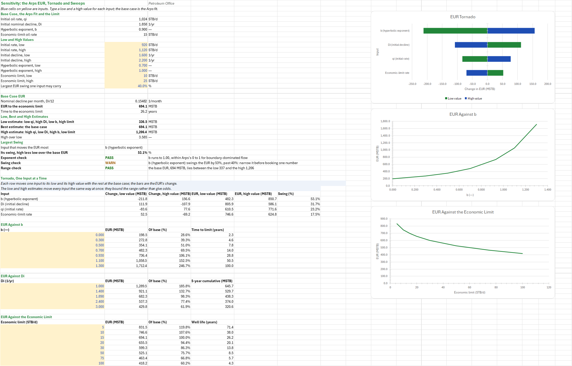
How much oil will this well recover, and how far can that number move? You paste one well's monthly oil rates; the workbook screens out the months that disagree with their neighbours, fits Arps, Duong, the power-law exponential (PLE) and the stretched exponential (SEDM) to the cleaned history, and forecasts each to an economic limit. You read off each model's EUR and life, the model to book, and how much each decline parameter moves the EUR. Field units; time in months, rates in STB/d.
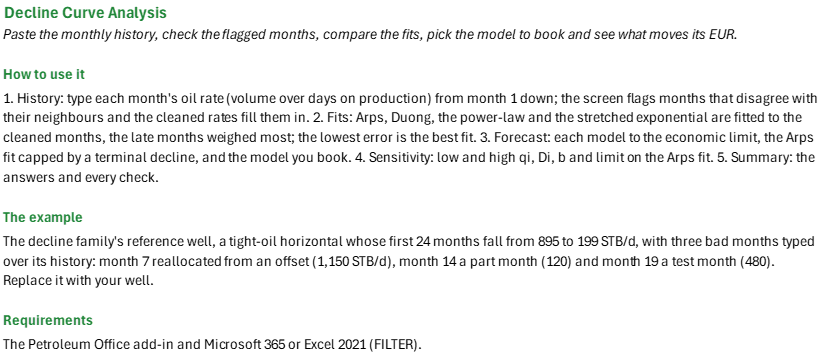
How to use it: Enter monthly volumes over days on production on the History sheet, from month 1 down with no gaps (up to 36 months). Check every flagged month against the field record (allocation, downtime, tests) before trusting its cleaned rate. On the Forecast sheet, take the terminal decline from older analogue wells and the economic limit from the operating cost over the netback, and pick the model to book. On the Sensitivity sheet, take the low and high values from the fit's spread or from analogues. The Summary gathers the answers and the checks.
Method: The screen flags a month whose rate lies more than a set number of standard deviations from its rolling window, and interpolates over it. Each model is fitted by Nelder-Mead to minimize the weighted log error sum w (ln q − ln q_fit)² over the typed months, with month t of a history ending at T weighed (t/T)^p; the History sheet's two Arps fits are unweighted. Arps q = qi/(1 + b Di t)^(1/b); Duong q = q1 t^−m exp(a/(1 − m) (t^(1−m) − 1)) + q∞; PLE q = qi exp(−D∞ t − Di t^n); SEDM q = qi exp(−(t/τ)^n). The secant effective decline is 1 − (1 + b Di)^(−1/b) with Di per year; the modified hyperbolic switches to an exponential at the terminal decline at t = (Di/Dlim − 1)/(b Di). Each model's EUR and life are its cumulative and time to the economic limit, the cumulative in STB/d·month times 30.4375 days a month. The tornado moves one input at a time; the low and high estimates move all four at once.
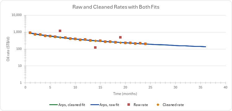
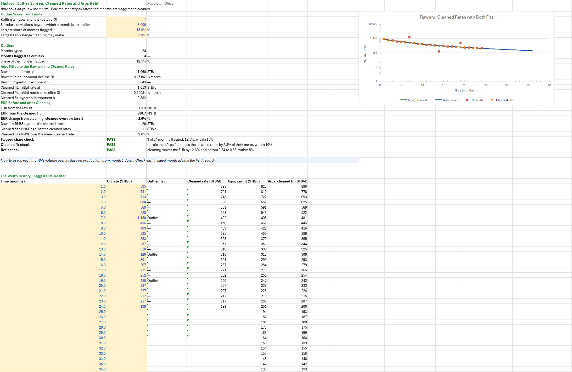
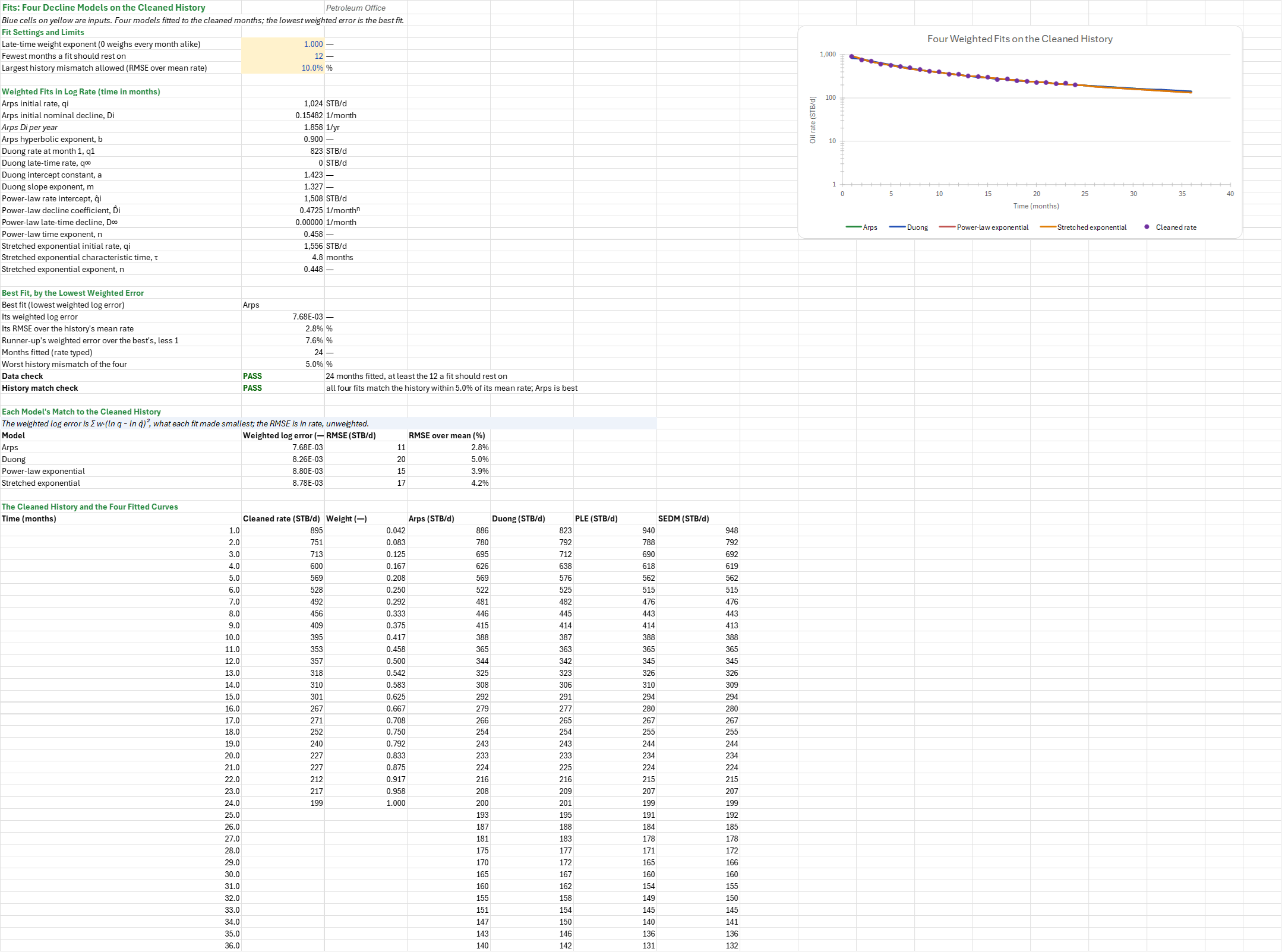
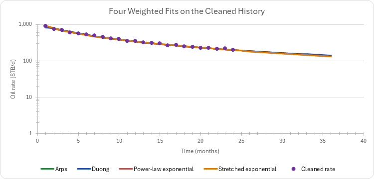
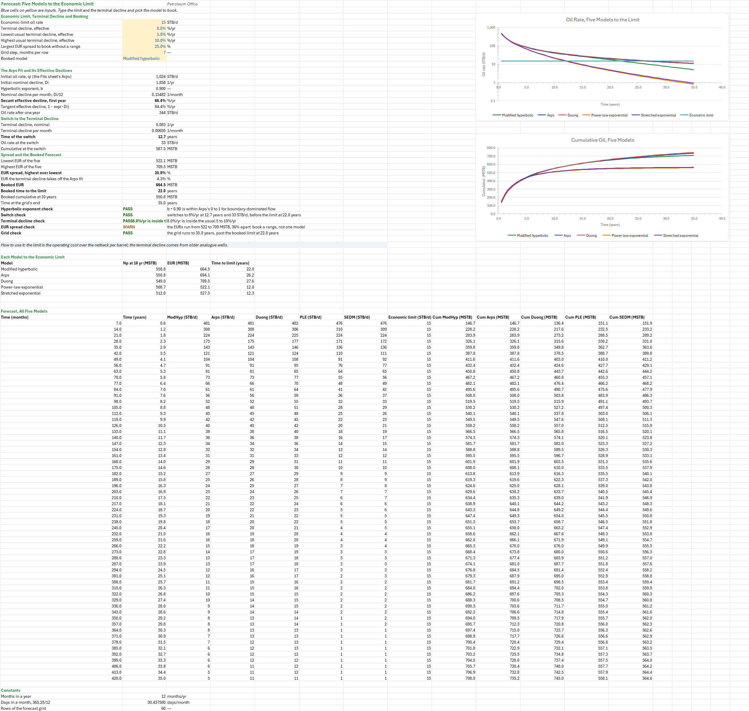
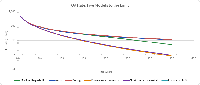
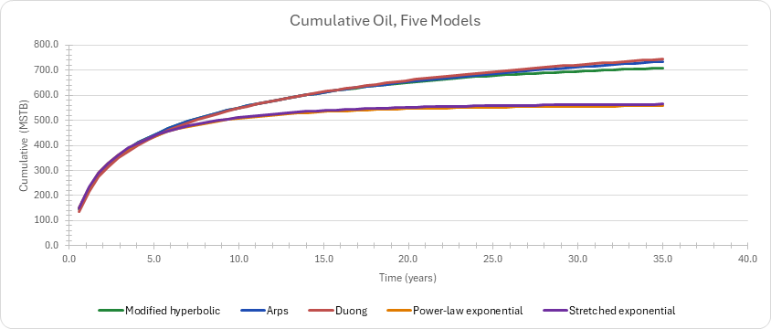
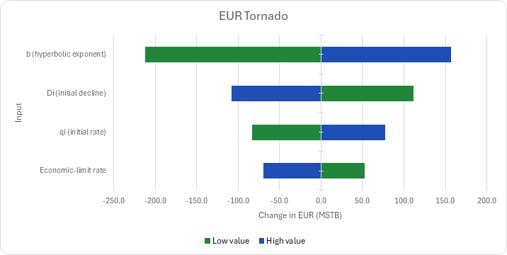
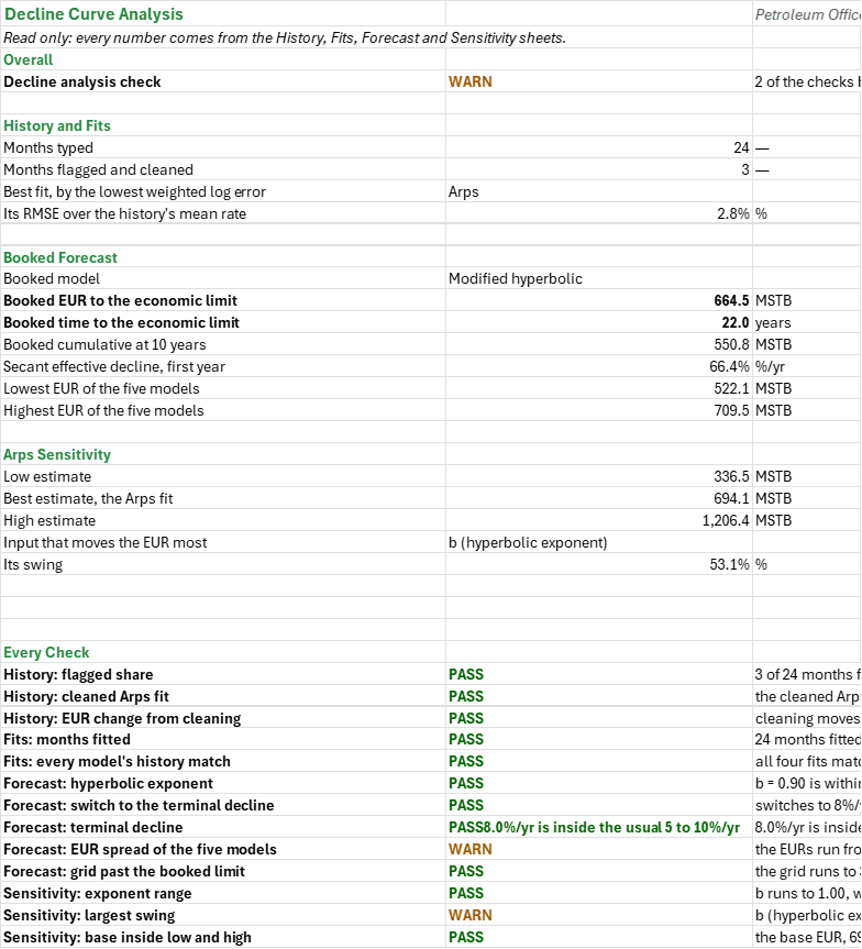
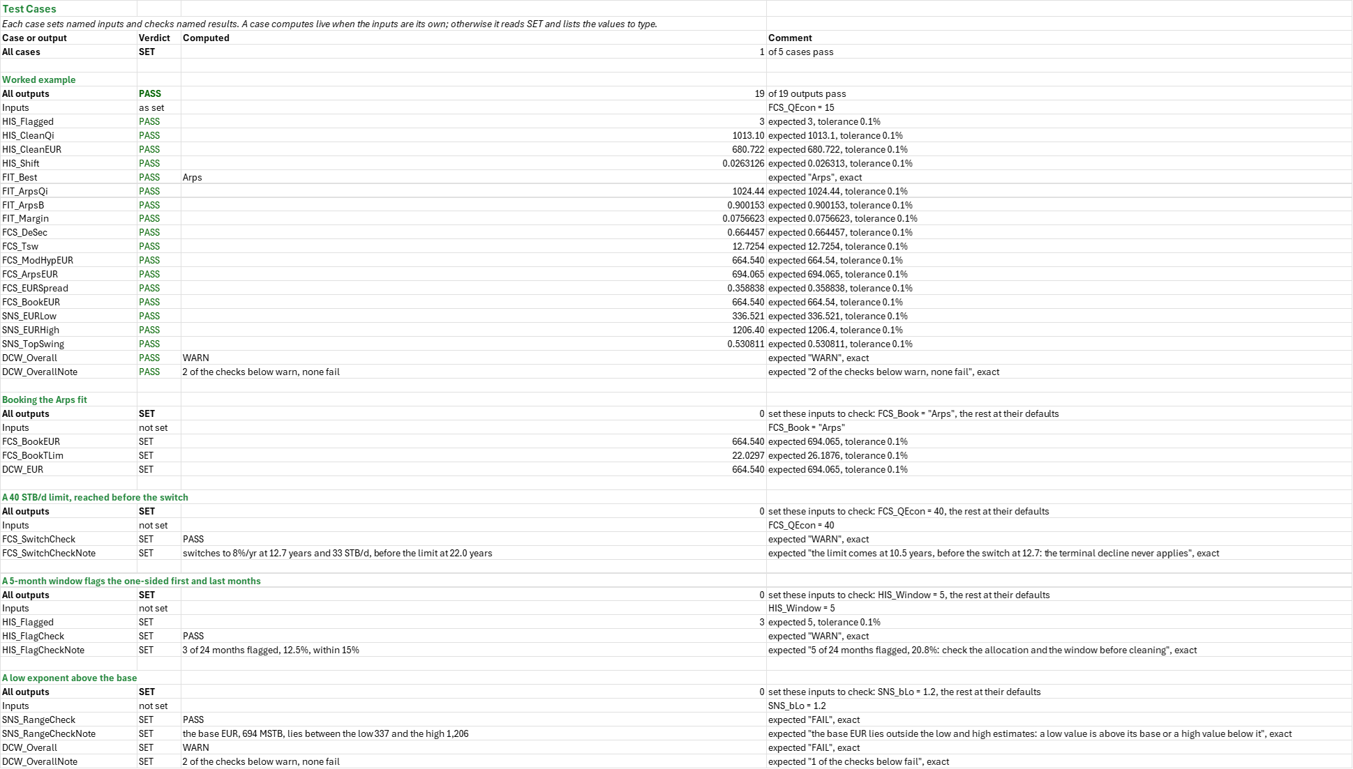
Example: The decline family's reference well (24 months from 895 to 199 STB/d) with three bad months typed over it: month 7 at 1,150 STB/d, 14 at 120 and 19 at 480. A 7-month window at 3 standard deviations flags exactly those three, 12.5 % of the months, and cleans them to 492, 309.5 and 239.5 STB/d. Arps fitted to the raw rates gives qi 1,060.4 STB/d, Di 0.15102/month and b 0.843; fitted to the cleaned rates, 1,013.1, 0.15034 and 0.882, with an RMSE of 2.8 % of the mean rate. Cleaning moves the EUR from 663.3 to 680.7 MSTB, +2.6 %, inside the 5 % allowed. With linear late-time weights the four fits score 0.007677 (Arps: qi 1,024.4, Di 1.858/yr, b 0.900), 0.008257 (Duong: q1 822.7, a 1.423, m 1.327), 0.008781 (SEDM: qi 1,556.1, τ 4.80 months, n 0.448) and 0.008795 (PLE: qi 1,508.0, Di 0.4725, n 0.458, with D∞ at its lower bound of zero). Arps is best by 7.6 %, and every fit matches the history within 5.0 % of the mean rate. The Arps fit declines 66.4 %/yr (secant) in its first year, to 343.7 STB/d. With the terminal decline at 8 %/yr it switches after 12.7 years at 32.6 STB/d. To 15 STB/d the EURs are 664.5 MSTB modified hyperbolic (22.0 years, the booked model), 694.1 Arps (26.2), 709.5 Duong (27.6), 527.5 SEDM (12.3) and 522.1 PLE (12.0). They lie 36 % apart, more than the 25 % allowed, so book a range. On the Arps fit, b moves the EUR most: 53 % from 0.7 to 1.0, more than the 40 % one input may carry. The low and high estimates are 336.5 and 1,206.4 MSTB, with the base case between them.
Validity
Decline models are empirical and hold at constant operating conditions; a workover, choke change or interference starts a new decline. A rolling Z-score can't tell a reporting error from a real event, and a run of bad months longer than half the window hides itself. The weighted fits favour the late months; on 24 months of a tight well's transient flow they agree within 5 % on the history and still differ by a third in EUR, which is the EUR spread the Forecast sheet reports. On this history the PLE fit takes D∞ to its lower bound of zero, so its forecast is close to SEDM's; a fixed D∞ needs a hand fit. Arps with b above 1 is transient and its EUR rests on the limit alone: book the modified hyperbolic. The sensitivity is Arps only and moves one input at a time, ignoring that a fit's qi, Di and b move together; the low and high estimates are deterministic scenarios, not P90/P10. Alternatives: rate-transient analysis or flowing material balance where pressures are measured, type wells from offsets, a Monte Carlo on the fit's covariance, AIC or BIC to penalize Duong's fourth parameter.
References
- Arps, J.J. (1945). Analysis of Decline Curves. Trans. AIME 160, 228-247.
- Fetkovich, M.J. (1980). Decline Curve Analysis Using Type Curves. JPT 32(6), 1065-1077.
- Robertson, S. (1988). Generalized Hyperbolic Equation. SPE-18731-MS.
- Ilk, D., Rushing, J.A., Perego, A.D. and Blasingame, T.A. (2008). Exponential vs. Hyperbolic Decline in Tight Gas Sands. SPE-116731-MS.
- Valko, P.P. and Lee, W.J. (2010). A Better Way to Forecast Production from Unconventional Gas Wells. SPE-134231-MS.
- Duong, A.N. (2011). Rate-Decline Analysis for Fracture-Dominated Shale Reservoirs. SPE Res Eval & Eng 14(3), 377-387.
- SPEE (2016). Monograph 4: Estimating Ultimate Recovery of Developed Wells in Low-Permeability Reservoirs.
Inputs
| Input | Unit | Default | Name |
|---|---|---|---|
| Monthly oil rate, months 1 to 36 | STB/d | reference well (24 months) with 3 bad months | HIS_Q |
| Rolling window, months (at least 3) | months | 7 | HIS_Window |
| Standard deviations beyond which a month is an outlier | — | 3 | HIS_NSigma |
| Largest share of months flagged | % | 15 | HIS_FlagMax |
| Largest EUR change cleaning may make | % | 5 | HIS_ShiftMax |
| Late-time weight exponent (0 weighs every month alike) | — | 1 | FIT_WPow |
| Fewest months a fit should rest on | months | 12 | FIT_MinMonths |
| Largest history mismatch allowed (RMSE over mean rate) | % | 10 | FIT_FitMax |
| Economic-limit oil rate | STB/d | 15 | FCS_QEcon |
| Terminal decline, effective | 1/yr | 0.08 | FCS_Dlim |
| Lowest and highest usual terminal decline, effective | 1/yr | 0.05, 0.10 | FCS_DlimLo, FCS_DlimHi |
| Largest EUR spread to book without a range | % | 25 | FCS_SpreadMax |
| Grid step, months per row | months | 7 | FCS_Step |
| Booked model (from a list) | — | Modified hyperbolic | FCS_Book |
| Initial rate, low and high | STB/d | 920, 1,120 | SNS_qiLo, SNS_qiHi |
| Initial decline, low and high | 1/yr | 1.6, 2.2 | SNS_DiLo, SNS_DiHi |
| Hyperbolic exponent, low and high | — | 0.7, 1.0 | SNS_bLo, SNS_bHi |
| Economic limit, low and high | STB/d | 10, 25 | SNS_QEconLo, SNS_QEconHi |
| Largest EUR swing one input may carry | % | 40 | SNS_SwingMax |
Sheets
Guide— what the workbook answers and the order to work through its sheets.History— the open table of months, a rolling Z-score that flags the months that disagree with their neighbours, the cleaned rates, and Arps fitted to the raw and the cleaned rates with each fit's EUR.Fits— Arps, Duong, PLE and SEDM fitted to the cleaned months in log rate with late-time weights, each fit's weighted log error and RMSE, and the best fit by the lowest error.Forecast— the Arps fit's secant and tangent effective declines and its switch to a terminal decline (the modified hyperbolic); the five models' 10-year cumulative, EUR and life to one economic limit with their spread; the model to book, picked from a list; a 35-year forecast grid with rate and cumulative charts.Sensitivity— the Arps EUR with a low and a high qi, Di, b and limit, a tornado, the low, best and high estimates, and sweeps of b, Di and the limit.Summary— the answers and every check under one verdict.Test Cases— the worked example and other cases, with expected and computed results.
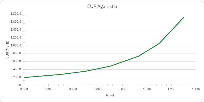
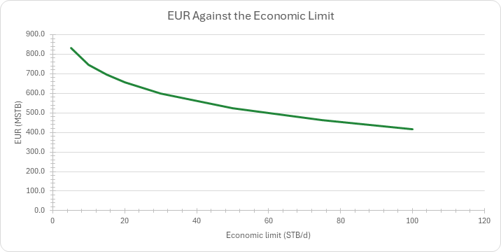
Seven charts: raw and cleaned rates with both Arps fits; the four weighted fits on the cleaned history; five models' rates to the limit; their cumulatives; the EUR tornado; the EUR against b; the EUR against the limit.
Functions used
Names (184)
| Name | Refers to | Comment |
|---|---|---|
PO.DCA.Arps.SecantEffLAMBDA |
=LAMBDA(Di, b, IF(OR(Di<0, b<0), NA(), IF(b=0, 1-EXP(-Di), 1-(1+b*Di)^(-1/b)))) |
Secant effective decline (fraction per period) of an Arps hyperbolic: 1 - (1 + b*Di)^(-1/b), or 1 - exp(-Di) for b = 0. Di is the nominal decline per period (1/yr gives the effective annual decline) and b the exponent. |
PO.DCA.ModHyp.TswitchLAMBDA |
=LAMBDA(Di, Dlim, b, IF(OR(Di<=0, Dlim<=0, b<=0), NA(), IF(Dlim>=Di, 0, (Di/Dlim-1)/(b*Di)))) |
Time a modified hyperbolic switches to its terminal exponential: (Di/Dlim - 1)/(b*Di), 0 when Dlim >= Di. Di and Dlim are nominal declines in one time base (1/month gives months) and b the hyperbolic exponent. |
DCW_Best |
Summary!$B$9 |
Best fit, by the lowest weighted log error |
DCW_BestRelErr |
Summary!$B$10 |
Its RMSE over the history's mean rate, % |
DCW_Book |
Summary!$B$13 |
Booked model |
DCW_Checks |
Summary!$B$31:$B$43 |
Every check of the workbook, read from its sheet |
DCW_DeSec |
Summary!$B$17 |
Secant effective decline, first year, %/yr |
DCW_EUR |
Summary!$B$14 |
Booked EUR to the economic limit, MSTB |
DCW_EURBest |
Summary!$B$23 |
Best estimate, the Arps fit, MSTB |
DCW_EURHi |
Summary!$B$19 |
Highest EUR of the five models, MSTB |
DCW_EURHigh |
Summary!$B$24 |
High estimate, MSTB |
DCW_EURLo |
Summary!$B$18 |
Lowest EUR of the five models, MSTB |
DCW_EURLow |
Summary!$B$22 |
Low estimate, MSTB |
DCW_Fit_Results |
Summary!$B$7:$B$10 |
The months typed and flagged, the best fit and its history mismatch |
DCW_Flagged |
Summary!$B$8 |
Months flagged and cleaned |
DCW_Forecast_Results |
Summary!$B$13:$B$19 |
The booked model, its EUR and life, and the spread of the five |
DCW_N |
Summary!$B$7 |
Months typed |
DCW_Np10 |
Summary!$B$16 |
Booked cumulative at 10 years, MSTB |
DCW_Overall |
Summary!$B$4 |
Decline analysis check verdict |
DCW_OverallNote |
Summary!$C$4 |
Decline analysis check comment |
DCW_Sensitivity_Results |
Summary!$B$22:$B$26 |
The low, best and high Arps EUR and the largest swing |
DCW_TLim |
Summary!$B$15 |
Booked time to the economic limit, years |
DCW_Top |
Summary!$B$25 |
Input that moves the EUR most |
DCW_TopSwing |
Summary!$B$26 |
Its swing, % |
DCW_Verdict |
Summary!$B$4 |
One verdict over every check of the workbook |
DCW_VerdictNote |
Summary!$C$4 |
One verdict over every check of the workbook comment |
FCS_ArpsEUR |
Forecast!$C$46 |
Arps EUR, MSTB |
FCS_BCheck |
Forecast!$B$35 |
Hyperbolic exponent check verdict |
FCS_BCheckNote |
Forecast!$C$35 |
Hyperbolic exponent check comment |
FCS_Book |
Forecast!$B$10 |
Booked model |
FCS_BookEUR |
Forecast!$B$31 |
Booked EUR, MSTB |
FCS_BookNp10 |
Forecast!$B$33 |
Booked cumulative at 10 years, MSTB |
FCS_BookTLim |
Forecast!$B$32 |
Booked time to the limit, years |
FCS_Curve |
Forecast!$A$54:$M$113 |
Time, each model's rate and cumulative, and the limit |
FCS_Cut |
Forecast!$B$30 |
EUR the terminal decline takes off the Arps fit, % |
FCS_DMo |
Forecast!$B$117 |
Days in a month, 365.25/12, days/month |
FCS_DeSec |
Forecast!$B$17 |
Secant effective decline, first year, %/yr |
FCS_DeTan |
Forecast!$B$18 |
Tangent effective decline, 1 − exp(−Di), %/yr |
FCS_Di |
Forecast!$B$14 |
Initial nominal decline, Di, 1/yr |
FCS_DiM |
Forecast!$B$16 |
Nominal decline per month, Di/12, 1/month |
FCS_Dlim |
Forecast!$B$5 |
Terminal decline, effective, %/yr |
FCS_DlimCheck |
Forecast!$B$37 |
Terminal decline check verdict |
FCS_DlimCheckNote |
Forecast!$C$37 |
Terminal decline check comment |
FCS_DlimHi |
Forecast!$B$7 |
Highest usual terminal decline, effective, %/yr |
FCS_DlimLo |
Forecast!$B$6 |
Lowest usual terminal decline, effective, %/yr |
FCS_DlimM |
Forecast!$B$22 |
Terminal decline per month, 1/month |
FCS_DlimN |
Forecast!$B$21 |
Terminal decline, nominal, 1/yr |
FCS_EURHi |
Forecast!$B$28 |
Highest EUR of the five, MSTB |
FCS_EURLo |
Forecast!$B$27 |
Lowest EUR of the five, MSTB |
FCS_EURSpread |
Forecast!$B$29 |
EUR spread, highest over lowest, % |
FCS_GridCheck |
Forecast!$B$39 |
Grid check verdict |
FCS_GridCheckNote |
Forecast!$C$39 |
Grid check comment |
FCS_GridEnd |
Forecast!$B$34 |
Time at the grid's end, years |
FCS_Inputs |
Forecast!$B$4:$B$10 |
The limit, the terminal decline and its range, the spread allowed, the step and the booked model |
FCS_MoYr |
Forecast!$B$116 |
Months in a year, months/yr |
FCS_ModHypEUR |
Forecast!$C$45 |
Modified hyperbolic EUR, MSTB |
FCS_ModHypTLim |
Forecast!$D$45 |
Modified hyperbolic time to the limit, years |
FCS_Models |
Forecast!$A$45:$D$49 |
Each model's 10-year cumulative, EUR and time to the limit |
FCS_NpSw |
Forecast!$B$25 |
Cumulative at the switch, MSTB |
FCS_QEcon |
Forecast!$B$4 |
Economic-limit oil rate, STB/d |
FCS_Results |
Forecast!$B$13:$B$39 |
The Arps fit and its declines, the switch, the EUR spread, the booked EUR and life, the grid's end and the five checks |
FCS_Rows |
Forecast!$B$118 |
Rows of the forecast grid |
FCS_SpreadCheck |
Forecast!$B$38 |
EUR spread check verdict |
FCS_SpreadCheckNote |
Forecast!$C$38 |
EUR spread check comment |
FCS_SpreadMax |
Forecast!$B$8 |
Largest EUR spread to book without a range, % |
FCS_Step |
Forecast!$B$9 |
Grid step, months per row |
FCS_SwitchCheck |
Forecast!$B$36 |
Switch check verdict |
FCS_SwitchCheckNote |
Forecast!$C$36 |
Switch check comment |
FCS_Tsw |
Forecast!$B$23 |
Time of the switch, years |
FCS_b |
Forecast!$B$15 |
Hyperbolic exponent, b |
FCS_q1yr |
Forecast!$B$19 |
Oil rate after one year, STB/d |
FCS_qSw |
Forecast!$B$24 |
Oil rate at the switch, STB/d |
FCS_qi |
Forecast!$B$13 |
Initial oil rate, qi (the Fits sheet's Arps), STB/d |
FIT_ArpsB |
Fits!$B$12 |
Arps hyperbolic exponent, b |
FIT_ArpsDi |
Fits!$B$11 |
Arps Di per year, 1/yr |
FIT_ArpsDiM |
Fits!$B$10 |
Arps initial nominal decline, Di, 1/month |
FIT_ArpsQi |
Fits!$B$9 |
Arps initial rate, qi, STB/d |
FIT_Best |
Fits!$B$26 |
Best fit (lowest weighted log error) |
FIT_BestErr |
Fits!$B$27 |
Its weighted log error |
FIT_BestRelErr |
Fits!$B$28 |
Its RMSE over the history's mean rate, % |
FIT_Curve |
Fits!$A$45:$G$80 |
The months, cleaned rates, weights and each fitted rate |
FIT_DataCheck |
Fits!$B$32 |
Data check verdict |
FIT_DataCheckNote |
Fits!$C$32 |
Data check comment |
FIT_DuongA |
Fits!$B$15 |
Duong intercept constant, a |
FIT_DuongM |
Fits!$B$16 |
Duong slope exponent, m |
FIT_DuongQ1 |
Fits!$B$13 |
Duong rate at month 1, q1, STB/d |
FIT_DuongQinf |
Fits!$B$14 |
Duong late-time rate, q∞, STB/d |
FIT_FitArps |
Fits!$D$45:$D$80 |
Arps fitted rate at each month, STB/d |
FIT_FitCheck |
Fits!$B$33 |
History match check verdict |
FIT_FitCheckNote |
Fits!$C$33 |
History match check comment |
FIT_FitDuong |
Fits!$E$45:$E$80 |
Duong fitted rate at each month, STB/d |
FIT_FitMax |
Fits!$B$6 |
Largest history mismatch allowed (RMSE over mean rate), % |
FIT_FitPLE |
Fits!$F$45:$F$80 |
Power-law exponential fitted rate at each month, STB/d |
FIT_FitSEDM |
Fits!$G$45:$G$80 |
Stretched exponential fitted rate at each month, STB/d |
FIT_Fits |
Fits!$B$9:$B$23 |
Each model's parameters fitted to the cleaned months |
FIT_Inputs |
Fits!$B$4:$B$6 |
The weight exponent, the fewest months and the mismatch allowed |
FIT_Margin |
Fits!$B$29 |
Runner-up's weighted error over the best's, less 1, % |
FIT_MinMonths |
Fits!$B$5 |
Fewest months a fit should rest on |
FIT_Models |
Fits!$A$38:$D$41 |
Each model's weighted log error and RMSE |
FIT_N |
Fits!$B$30 |
Months fitted (rate typed) |
FIT_PleDi |
Fits!$B$18 |
Power-law decline coefficient, D̂i, 1/monthⁿ |
FIT_PleDinfM |
Fits!$B$19 |
Power-law late-time decline, D∞, 1/month |
FIT_PleN |
Fits!$B$20 |
Power-law time exponent, n |
FIT_PleQi |
Fits!$B$17 |
Power-law rate intercept, q̂i, STB/d |
FIT_Results |
Fits!$B$26:$B$33 |
The best fit, its error, mismatch and margin, the months fitted, the worst mismatch and two checks |
FIT_SedmN |
Fits!$B$23 |
Stretched exponential exponent, n |
FIT_SedmQi |
Fits!$B$21 |
Stretched exponential initial rate, qi, STB/d |
FIT_SedmTau |
Fits!$B$22 |
Stretched exponential characteristic time, τ, months |
FIT_W |
Fits!$C$45:$C$80 |
Each month's late-time weight, (t/T)^WPow |
FIT_WPow |
Fits!$B$4 |
Late-time weight exponent (0 weighs every month alike) |
FIT_WorstFit |
Fits!$B$31 |
Worst history mismatch of the four, % |
HIS_Clean |
History!$D$36:$D$71 |
Cleaned rate (STB/d) |
HIS_CleanB |
History!$B$19 |
Cleaned fit, hyperbolic exponent b |
HIS_CleanDi |
History!$B$18 |
Cleaned fit, initial nominal decline Di, 1/month |
HIS_CleanEUR |
History!$B$22 |
EUR from the cleaned fit, MSTB |
HIS_CleanFit |
History!$F$36:$F$71 |
Arps, cleaned fit (STB/d) |
HIS_CleanQi |
History!$B$17 |
Cleaned fit, initial rate qi, STB/d |
HIS_CleanRMSE |
History!$B$25 |
Cleaned fit's RMSE against the cleaned rates, STB/d |
HIS_Curve |
History!$A$36:$F$71 |
Raw and Cleaned Rates with Both Fits |
HIS_FitCheck |
History!$B$28 |
Cleaned fit check verdict |
HIS_FitCheckNote |
History!$C$28 |
Cleaned fit check comment |
HIS_Fits |
History!$B$14:$B$19 |
Arps qi, Di and b fitted to the raw and to the cleaned rates |
HIS_Flag |
History!$C$36:$C$71 |
Outlier flag |
HIS_FlagCheck |
History!$B$27 |
Flagged share check verdict |
HIS_FlagCheckNote |
History!$C$27 |
Flagged share check comment |
HIS_FlagMax |
History!$B$6 |
Largest share of months flagged, % |
HIS_FlagShare |
History!$B$12 |
Share of the months flagged, % |
HIS_Flagged |
History!$B$11 |
Months flagged as outliers |
HIS_History |
History!$A$36:$F$71 |
The well's months, its oil rate typed for each month it has, empty months below for more, and the columns computed from them |
HIS_Inputs |
History!$B$4:$B$7 |
The screen's window and threshold and the two limits |
HIS_N |
History!$B$10 |
Months typed |
HIS_NSigma |
History!$B$5 |
Standard deviations beyond which a month is an outlier |
HIS_Outliers |
History!$B$10:$B$12 |
The months typed and flagged and the flagged share |
HIS_Q |
History!$B$36:$B$71 |
History oil rates, STB/d; an empty month is left out of the fits |
HIS_RawB |
History!$B$16 |
Raw fit, hyperbolic exponent b |
HIS_RawDi |
History!$B$15 |
Raw fit, initial nominal decline Di, 1/month |
HIS_RawEUR |
History!$B$21 |
EUR from the raw fit, MSTB |
HIS_RawFit |
History!$E$36:$E$71 |
Arps, raw fit (STB/d) |
HIS_RawQi |
History!$B$14 |
Raw fit, initial rate qi, STB/d |
HIS_RawRMSE |
History!$B$24 |
Raw fit's RMSE against the cleaned rates, STB/d |
HIS_RefitCheck |
History!$B$29 |
Refit check verdict |
HIS_RefitCheckNote |
History!$C$29 |
Refit check comment |
HIS_RelErr |
History!$B$26 |
Cleaned fit's RMSE over the mean cleaned rate, % |
HIS_Results |
History!$B$21:$B$29 |
Each fit's EUR, the change cleaning makes, each fit's RMSE against the cleaned rates, and the three checks |
HIS_Shift |
History!$B$23 |
EUR change from cleaning, cleaned over raw less 1, % |
HIS_ShiftMax |
History!$B$7 |
Largest EUR change cleaning may make, % |
HIS_T |
History!$A$36:$A$71 |
History months, 1 to 36 |
HIS_Window |
History!$B$4 |
Rolling window, months (at least 3) |
SNS_BCheck |
Sensitivity!$B$31 |
Exponent check verdict |
SNS_BCheckNote |
Sensitivity!$C$31 |
Exponent check comment |
SNS_B_Curve |
Sensitivity!$A$46:$D$52 |
The EUR, its share of the base and the time to the limit at each b, the rest at the base case |
SNS_Base |
Sensitivity!$B$4:$B$7 |
The Arps fit and the limit |
SNS_Di |
Sensitivity!$B$5 |
Initial nominal decline, Di, 1/yr |
SNS_DiHi |
Sensitivity!$B$12 |
Initial decline, high, 1/yr |
SNS_DiLo |
Sensitivity!$B$11 |
Initial decline, low, 1/yr |
SNS_DiM |
Sensitivity!$B$20 |
Nominal decline per month, Di/12, 1/month |
SNS_DiSweep |
Sensitivity!$A$56:$D$60 |
The EUR, its share of the base and the 5-year cumulative at each Di, the rest at the base case |
SNS_EUR |
Sensitivity!$B$21 |
EUR to the economic limit, MSTB |
SNS_EURBest |
Sensitivity!$B$25 |
Best estimate: the base case, MSTB |
SNS_EURHigh |
Sensitivity!$B$26 |
High estimate: high qi, low Di, high b, low limit, MSTB |
SNS_EURLow |
Sensitivity!$B$24 |
Low estimate: low qi, high Di, low b, high limit, MSTB |
SNS_HiLo |
Sensitivity!$B$27 |
High over low |
SNS_Inputs |
Sensitivity!$B$9:$B$17 |
Low and high qi, Di, b and limit, and the swing allowed |
SNS_Limit_Curve |
Sensitivity!$A$64:$D$71 |
The EUR, its share of the base and the well's life at each economic-limit rate, the rest at the base case |
SNS_QEcon |
Sensitivity!$B$7 |
Economic-limit oil rate, STB/d |
SNS_QEconHi |
Sensitivity!$B$16 |
Economic limit, high, STB/d |
SNS_QEconLo |
Sensitivity!$B$15 |
Economic limit, low, STB/d |
SNS_RangeCheck |
Sensitivity!$B$33 |
Range check verdict |
SNS_RangeCheckNote |
Sensitivity!$C$33 |
Range check comment |
SNS_Results |
Sensitivity!$B$20:$B$33 |
The base EUR and life, the low, best and high estimates, the largest swing and three checks |
SNS_SwingCheck |
Sensitivity!$B$32 |
Swing check verdict |
SNS_SwingCheckNote |
Sensitivity!$C$32 |
Swing check comment |
SNS_SwingMax |
Sensitivity!$B$17 |
Largest EUR swing one input may carry, % |
SNS_TLim |
Sensitivity!$B$22 |
Time to the economic limit, years |
SNS_Top |
Sensitivity!$B$29 |
Input that moves the EUR most |
SNS_TopSwing |
Sensitivity!$B$30 |
Its swing, high less low over the base EUR, % |
SNS_Tornado |
Sensitivity!$A$39:$F$42 |
Each input's EUR change at its low and high value, and its swing |
SNS_Tornado_Curve |
Sensitivity!$A$39:$C$42 |
EUR Tornado |
SNS_b |
Sensitivity!$B$6 |
Hyperbolic exponent, b |
SNS_bHi |
Sensitivity!$B$14 |
Hyperbolic exponent, high |
SNS_bLo |
Sensitivity!$B$13 |
Hyperbolic exponent, low |
SNS_qi |
Sensitivity!$B$4 |
Initial oil rate, qi, STB/d |
SNS_qiHi |
Sensitivity!$B$10 |
Initial rate, high, STB/d |
SNS_qiLo |
Sensitivity!$B$9 |
Initial rate, low, STB/d |
Details
| Opens in | Needs the Petroleum Office add-in: its PO functions show #NAME? without it once Excel recalculates. Needs Microsoft 365 or Excel 2024: it uses functions Excel 2016 doesn't have, such as named LAMBDAs, which show #NAME? there. |
| File | DeclineAnalysis.xlsx, 107 KB |
| Category | Production |
| For agents and tools | Descriptor (.md) |