Well Test Design
Description
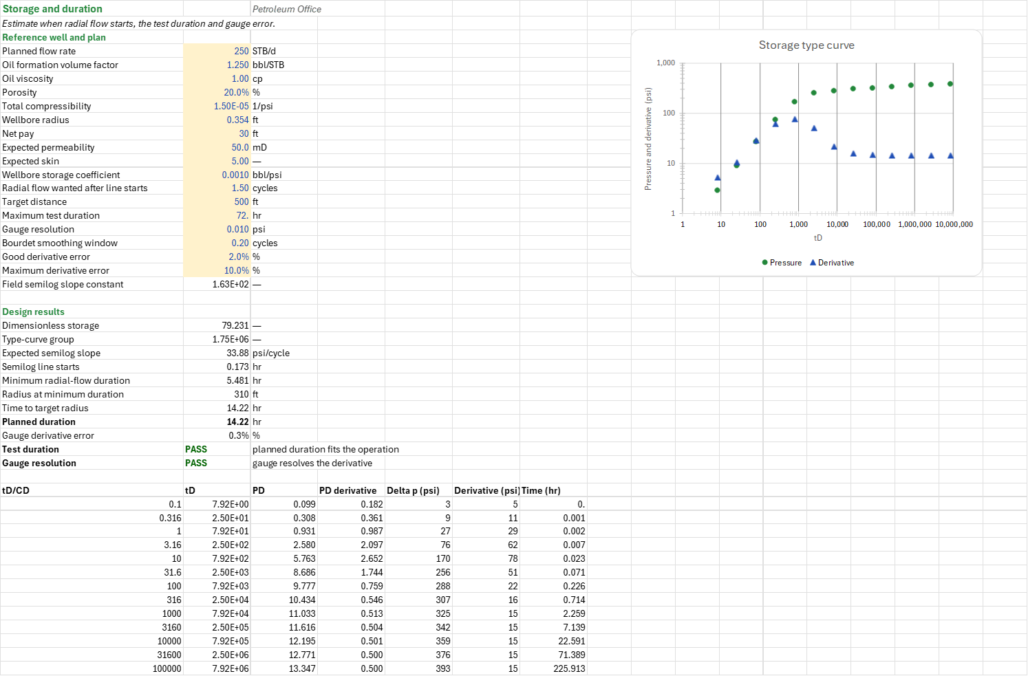
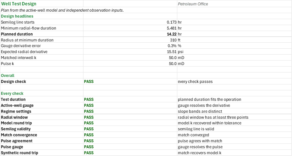
How long must a planned well test run to see radial flow and reach a target radius, will the gauge resolve the derivative, and what would an observation well record? You enter the rate, fluid and rock from the planned operation and offset tests, the target distance and the gauge resolution. You read off when the semilog line starts, the planned duration, the gauge derivative error, the expected derivative near a fault, and the observation well's matched and pulse permeability. Field units; time in hours.
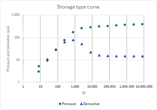
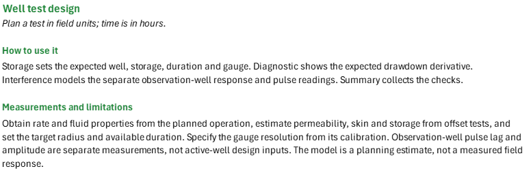
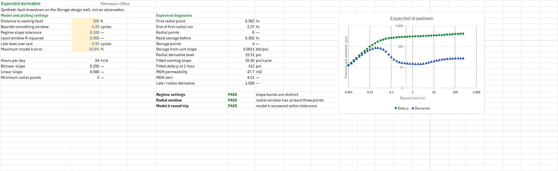
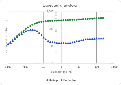
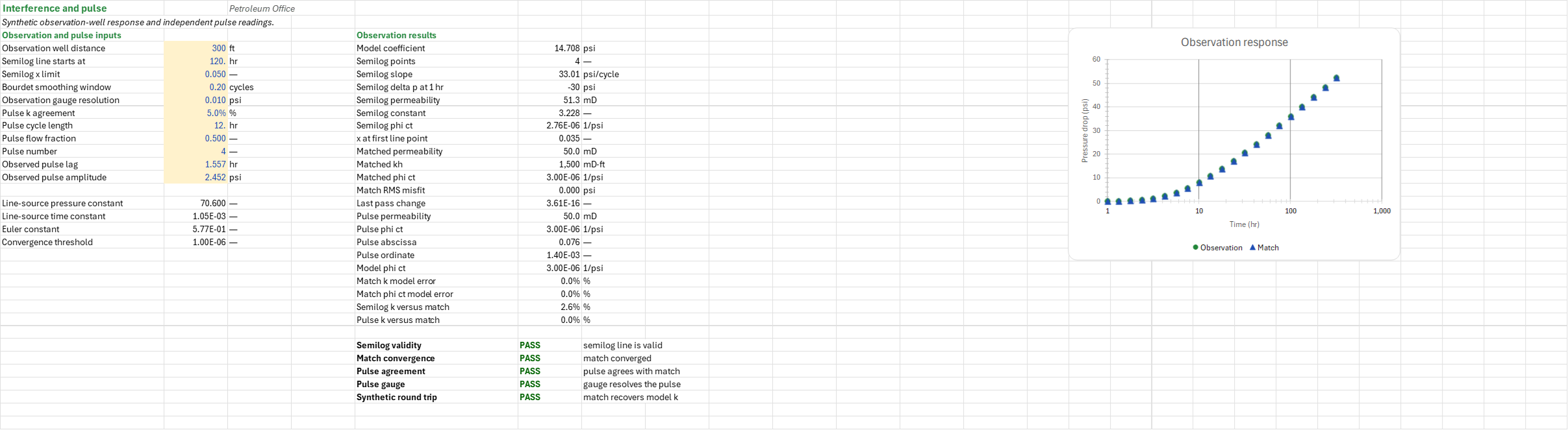
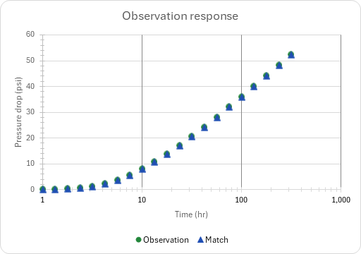
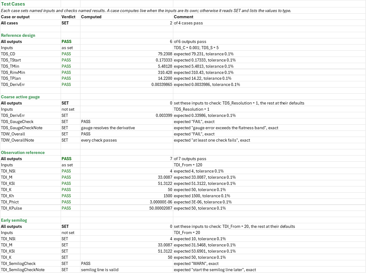
How to use it: Take the rate and fluid properties from the proposed operation, and the permeability, skin and storage from offset tests or the completion design, on the Storage sheet; set the target radius, the hours available and the gauge resolution from its calibration. The planned duration is the longer of the time needed for radial flow and the time to the target radius. A derivative gauge error above the acceptable band calls for a finer gauge or a wider smoothing window. The Diagnostic sheet shows the drawdown and derivative to expect on the same well. For interference, set the observation-well spacing on the Interference sheet and plan drift-corrected pressure readings over time. Pulse lag is measured from the end of the pulse to its extremum, and amplitude from the tangent to the neighbouring extrema; here they are independent observation inputs, not a prediction of the active-well storage model. To analyse an observation record instead of the example, paste its 21 positive, increasing time and drift-corrected pressure-drop pairs into Interference A47:B67; other row counts need the dependent ranges and formulas resized. The Summary lists every check.
Method: The dimensionless storage CD and the type-curve group CD e^(2S) set the storage type curve. The expected semilog slope is m = 162.6 q B μ/(k h). Earlougher's rule puts the start of the semilog line at t = (200000 + 12000 S) C μ/(k h), and the minimum radial-flow duration at that times 10^cycles. The radius of investigation follows from k, t, φ, μ and ct, and its inverse gives the time to the target radius. The gauge derivative error follows from the gauge resolution, the semilog slope and the Bourdet smoothing window. The diagnostic is a synthetic drawdown near a sealing fault with its Bourdet derivative, regime windows picked over five points and an MDH semilog fit. The interference model is the line source Δp = 70.6 q B μ/(k h) E1(x), with x = φ μ ct r^2/(0.0010548 k t); it is fitted by a semilog line and by four Gauss-Newton passes on permeability and φ ct. The pulse analysis reads permeability and φ ct from the pulse lag and amplitude.
Example: The reference plan: 250 STB/d, Bo 1.25, viscosity 1 cP, porosity 0.2, compressibility 1.5e-5/psi, rw 0.354 ft, pay 30 ft, k 50 mD, skin 5 and storage 0.001 bbl/psi. It needs about 14.22 h to reach 500 ft. The diagnostic is a model 200 ft from a sealing fault. The observation well is 300 ft away; its default pulse lag and amplitude are synthetic example readings, not field data.
Validity
Single-phase, constant-property flow in a homogeneous reservoir is assumed. Storage duration is empirical; variable storage, fractures, boundaries and noise change the derivative. The diagnostic is a synthetic drawdown, not a measured gauge or an interpretation of real data. The interference line-source model assumes a constant active-well rate, an infinite isotropic reservoir and a non-flowing observation well. A semilog line needs small x; pulse analysis needs drift-corrected readings and a pulse number of at least two. Active-well storage and skin are not included in the interwell line source.
The workbook does not compute, and the add-in has no functions for, the vertical-well type-curve fit, infinite-conductivity and uniform-flux fracture models, the horizontal-well model, finite-conductivity fracture modelling, interference type curves including active-well storage and skin, anisotropic interference and nonlinear boundary matching.
References
- Earlougher, R.C. Jr. (1977). Advances in Well Test Analysis. SPE Monograph 5.
- Kamal, M. and Brigham, W.E. (1975). Pulse-Testing Response for Unequal Pulse and Shut-In Periods. SPE Journal.
- Bourdet, D., Ayoub, J.A. and Pirard, Y.M. (1989). Use of Pressure Derivative in Well-Test Interpretation. SPE-12777-PA.
Inputs
| Input | Unit | Default | Name |
|---|---|---|---|
| Planned flow rate | STB/d | 250 | TDS_q |
| Oil formation volume factor | bbl/STB | 1.25 | TDS_Bo |
| Oil viscosity | cP | 1 | TDS_Mu |
| Porosity | fraction | 0.2 | TDS_Phi |
| Total compressibility | 1/psi | 0.000015 | TDS_Ct |
| Wellbore radius | ft | 0.354 | TDS_Rw |
| Net pay | ft | 30 | TDS_Pay |
| Expected permeability | mD | 50 | TDS_K |
| Expected skin | dimensionless | 5 | TDS_S |
| Wellbore storage coefficient | bbl/psi | 0.001 | TDS_C |
| Radial flow wanted after line starts | log cycles | 1.5 | TDS_Cycles |
| Target distance | ft | 500 | TDS_RTarget |
| Maximum test duration | h | 72 | TDS_MaxHours |
| Gauge resolution | psi | 0.01 | TDS_Resolution |
| Bourdet smoothing window; good and maximum derivative error | log cycles, % | see the Storage sheet | TDS_L, TDS_GoodErr, TDS_MaxErr |
| Distance to sealing fault | ft | 200 | TDD_Lb |
| Bourdet smoothing window | log cycles | 0.2 | TDD_L |
| Regime slope tolerance | fraction | 0.1 | TDD_Tol |
| Least window R-squared | fraction | 0.98 | TDD_R2 |
| Late level over last | log cycles | 0.5 | TDD_Span |
| Maximum model k error | fraction | 0.1 | TDD_KTol |
| Observation well distance | ft | 300 | TDI_r |
| Semilog line starts at | h | 120 | TDI_From |
| Observation gauge resolution | psi | 0.01 | TDI_Res |
| Semilog x limit; Bourdet smoothing window; pulse k agreement | —, log cycles, % | see the Interference sheet | TDI_xMax, TDI_L, TDI_KTol |
| Pulse cycle length | h | 12 | TDI_dtC |
| Pulse flow fraction | fraction | 0.5 | TDI_Fp |
| Pulse number | count | 4 | TDI_n |
| Observed pulse lag | h | 1.557117 | TDI_tL |
| Observed pulse amplitude | psi | 2.451508 | TDI_PDp |
Sheets
Guide— what the workbook plans, how to use it, and the measurements and limitations.Storage— the reference well and plan; when the semilog line starts, the minimum radial-flow duration, the radius at that time, the time to the target radius, the planned duration and the gauge derivative error, with the storage type curve.Diagnostic— a synthetic drawdown 200 ft from a sealing fault on the Storage well with its Bourdet derivative, the regime windows and the expected radial derivative.Interference— the observation-well response from the line source, its semilog fit and the Gauss-Newton match for permeability and φ ct, and the pulse-test analysis.Summary— the design headlines and every check under one verdict.Test Cases— the worked example and other cases, with expected and computed results.
Functions used
Names (133)
| Name | Refers to | Comment |
|---|---|---|
PO.PTA.Design.DurationLAMBDA |
=LAMBDA(C, mu, k, h, S, cycles, IF((200000+12000*S)*C*mu/(k*h)<=0, NA(), (200000+12000*S)*C*mu/(k*h)*10^cycles)) |
Test duration: the start of the semilog straight line, (200000 + 12000·S)·C·μ/(k·h), carried cycles log cycles further; cycles = 0 gives the start of the line itself, [h]. |
PO.PTA.Design.GaugeResLAMBDA |
=LAMBDA(m, resolution, L, IF(OR(m<=0, L<=0), NA(), LN(10)*resolution/(L*m))) |
Gauge-resolution check: the worst-case error that a gauge resolution puts into a Bourdet derivative over a smoothing window L, as a fraction of the radial-flow derivative m/ln(10): ln(10)·resolution/(L·m), [fraction]. |
PO.PTA.Design.RinvLAMBDA |
=LAMBDA(k, t, phi, mu, ct, SQRT(k*t/(948*phi*mu*ct))) |
Radius of investigation of radial flow after t hours: sqrt(k·t / (948·φ·μ·ct)), [ft]. |
PO.PTA.MDH.FitLAMBDA |
=LAMBDA(t, dp, q, B, mu, h, phi, ct, rw, output, LET(x, LOG10(t), m, SLOPE(dp, x), dp_1h, INTERCEPT(dp, x), perm, 162.6*q*B*mu/(m*h), skin, 1.151*(dp_1h/m-LOG10(perm/(phi*mu*ct*rw^2))+3.23), IF(m<=0, NA(), IF(output="k", perm, IF(output="S", skin, IF(output="m", m, IF(output="dp1h", dp_1h, NA()))))))) |
MDH semilog straight-line fit of a drawdown: least squares of Δp against log10(t) over the points given; output "k" [mD], "S" [dimensionless], "m" [psi/cycle] or "dp1h" [psi], the line's Δp at 1 h. |
PO.PTA.Pulse.AnalysisLAMBDA |
=LAMBDA(tL, dp, dtC, Fp, n, q, B, mu, h, robs, output, IF(OR(n<2, n<>ROUND(n, 0), Fp<=0, Fp>=1, tL<=0, dp<=0, dtC<=0), NA(), LET(lam, tL/dtC, nn, 600, jc, SEQUENCE(n+2, 1, 0), xs, jc/2+(Fp-0.5)*(1-(-1)^jc)/2, sgc, (-1)^jc, sgn, (-1)^(n+1), xepv, (n-1)/2+(Fp-0.5)*(1-(-1)^(n-1))/2, xen, n/2+(Fp-0.5)*(1-(-1)^n)/2, xenx, (n+1)/2+(Fp-0.5)*(1-(-1)^(n+1))/2, xenn, (n+2)/2+(Fp-0.5)*(1-(-1)^(n+2))/2, ig, SEQUENCE(nn+1, 1, 0), wz, xenx-xen, dz, xen+wz*ig/nn-TRANSPOSE(xs), pos, (dz>0)*1, dzc, pos*dz+1-pos, lgc, REDUCE(-9, SEQUENCE(121), LAMBDA(acc, i, IF(acc>-9, acc, LET(aa, 10^(-3.05+0.05*i), dv, MMULT(pos*EXP(-aa/(4*dzc))/dzc, sgc), cnt, SUM((dv*sgn>0)*1), da, SUM((ig=cnt-1)*dv), db, SUM((ig=cnt)*dv), lagx, IF(OR(cnt=0, cnt>nn), 2, wz*(cnt-1+da/(da-db))/nn), IF(lagx>=lam, -3.05+0.05*i, -9))))), lg, REDUCE(lgc-0.05, SEQUENCE(30), LAMBDA(acc, i, LET(aa, 10^(acc+0.05/2^i), dv, MMULT(pos*EXP(-aa/(4*dzc))/dzc, sgc), cnt, SUM((dv*sgn>0)*1), da, SUM((ig=cnt-1)*dv), db, SUM((ig=cnt)*dv), lagx, IF(OR(cnt=0, cnt>nn), 2, wz*(cnt-1+da/(da-db))/nn), acc+IF(lagx<lam, 0.05/2^i, 0)))), la, 10^lg, lagf, LET(aa, la, dv, MMULT(pos*EXP(-aa/(4*dzc))/dzc, sgc), cnt, SUM((dv*sgn>0)*1), da, SUM((ig=cnt-1)*dv), db, SUM((ig=cnt)*dv), lagx, IF(OR(cnt=0, cnt>nn), 2, wz*(cnt-1+da/(da-db))/nn), lagx), ik, SEQUENCE(2*nn+1), inw, (ik<=nn)*1, inx, (ik>nn)*(ik<=2*nn), atc, (ik>2*nn)*1, gx, inw*(xepv+(xen-xepv)*ik/nn)+inx*(xenx+(xenn-xenx)*(ik-nn)/nn)+atc*(xen+lam), dx, gx-TRANSPOSE(xs), px, (dx>0)*1, zx, la/(4*(px*dx+1-px)), lo, (zx<=1)*1, eone, lo*(-LN(zx)-0.57721566+zx*(0.99999193+zx*(-0.24991055+zx*(0.05519968+zx*(-0.00976004+zx*0.00107857)))))+(1-lo)*EXP(0-zx)/zx*(zx^4+8.5733287401*zx^3+18.059016973*zx^2+8.6347608925*zx+0.2677737343)/(zx^4+9.5733223454*zx^3+25.6329561486*zx^2+21.0996530827*zx+3.9584969228), pdx, MMULT(px*eone, sgc)/2, big, 10^300, sl, REDUCE(0, SEQUENCE(60), LAMBDA(acc, i, LET(v, sgn*(pdx-acc*gx), f, MIN(v+(1-inw)*big)-MIN(v+(1-inx)*big), acc+IF(sgn*f<0, 1, -1)*100/2^i))), base, sgn*MIN(sgn*(pdx-sl*gx)+(1-inw)*big), ad, ABS(SUM(atc*pdx)-base-sl*(xen+lam)), perm, 141.2*q*B*mu*ad/(h*dp), IF(OR(lgc<-2.99, ABS(lagf-lam)>0.0001*lam), NA(), IF(output="k", perm, IF(output="phict", 0.0002637*perm*la*dtC/(mu*robs^2), IF(output="tLD", lam/la, IF(output="dpD", ad*lam^2, NA())))))))) |
Kamal-Brigham pulse test from the time lag and amplitude of pulse n (≥ 2) on the line-source response; output "k" [md], "phict" [1/psi], "tLD" (tL)D/rD² or "dpD" ΔpD·(tL/ΔtC)², the chart ordinates. |
TDD_Before |
Diagnostic!$F$7 |
Read storage before, hr |
TDD_Cfit |
Diagnostic!$F$9 |
Storage from unit slope, bbl/psi |
TDD_Curve |
Diagnostic!$A$34:$C$77 |
Expected drawdown |
TDD_Dp1h |
Diagnostic!$F$12 |
Fitted delta p at 1 hour, psi |
TDD_Hr |
Diagnostic!$B$11 |
Hours per day, hr/d |
TDD_Inputs |
Diagnostic!$B$4:$B$9 |
Diagnostic settings; reference well is linked to Storage |
TDD_K |
Diagnostic!$F$13 |
MDH permeability, mD |
TDD_KTol |
Diagnostic!$B$9 |
Maximum model k error, % |
TDD_L |
Diagnostic!$B$5 |
Bourdet smoothing window, cycles |
TDD_Lb |
Diagnostic!$B$4 |
Distance to sealing fault, ft |
TDD_Level |
Diagnostic!$F$10 |
Radial derivative level, psi |
TDD_M |
Diagnostic!$F$11 |
Fitted semilog slope, psi/cycle |
TDD_MinN |
Diagnostic!$B$14 |
Minimum radial points |
TDD_ModelCheck |
Diagnostic!$F$19 |
Model k round trip verdict |
TDD_ModelCheckNote |
Diagnostic!$G$19 |
Model k round trip comment |
TDD_NRad |
Diagnostic!$F$6 |
Radial points |
TDD_NSto |
Diagnostic!$F$8 |
Storage points |
TDD_R2 |
Diagnostic!$B$7 |
Least window R-squared |
TDD_RadEnd |
Diagnostic!$F$5 |
End of first radial run, hr |
TDD_RadStart |
Diagnostic!$F$4 |
First radial point, hr |
TDD_Ratio |
Diagnostic!$F$15 |
Late / radial derivative |
TDD_RegimeCheck |
Diagnostic!$F$18 |
Radial window verdict |
TDD_RegimeCheckNote |
Diagnostic!$G$18 |
Radial window comment |
TDD_Results |
Diagnostic!$F$4:$F$19 |
Expected diagnostic results and checks |
TDD_S |
Diagnostic!$F$14 |
MDH skin |
TDD_SBil |
Diagnostic!$B$12 |
Bilinear slope |
TDD_SLin |
Diagnostic!$B$13 |
Linear slope |
TDD_SettingsCheck |
Diagnostic!$F$17 |
Regime settings verdict |
TDD_SettingsCheckNote |
Diagnostic!$G$17 |
Regime settings comment |
TDD_Span |
Diagnostic!$B$8 |
Late level over last, cycles |
TDD_Tol |
Diagnostic!$B$6 |
Regime slope tolerance |
TDI_AModel |
Interference!$F$4 |
Model coefficient, psi |
TDI_Conv |
Interference!$F$16 |
Last pass change |
TDI_ConvTol |
Interference!$B$19 |
Convergence threshold |
TDI_Curve |
Interference!$A$47:$M$67 |
Observation response |
TDI_Dp1h |
Interference!$F$7 |
Semilog delta p at 1 hr, psi |
TDI_DpD |
Interference!$F$20 |
Pulse ordinate |
TDI_Euler |
Interference!$B$18 |
Euler constant |
TDI_Fp |
Interference!$B$11 |
Pulse flow fraction |
TDI_From |
Interference!$B$5 |
Semilog line starts at, hr |
TDI_GaugeCheck |
Interference!$F$30 |
Pulse gauge verdict |
TDI_GaugeCheckNote |
Interference!$G$30 |
Pulse gauge comment |
TDI_Inputs |
Interference!$B$4:$B$14 |
Observation geometry, analysis and pulse readings; independent of the active-well storage plan |
TDI_K |
Interference!$F$12 |
Matched permeability, mD |
TDI_KErr |
Interference!$F$22 |
Match k model error, % |
TDI_KPulse |
Interference!$F$17 |
Pulse permeability, mD |
TDI_KSl |
Interference!$F$8 |
Semilog permeability, mD |
TDI_KTol |
Interference!$B$9 |
Pulse k agreement, % |
TDI_Kh |
Interference!$F$13 |
Matched kh, mD·ft |
TDI_L |
Interference!$B$7 |
Bourdet smoothing window, cycles |
TDI_LsC |
Interference!$F$9 |
Semilog constant |
TDI_M |
Interference!$F$6 |
Semilog slope, psi/cycle |
TDI_MatchCheck |
Interference!$F$28 |
Match convergence verdict |
TDI_MatchCheckNote |
Interference!$G$28 |
Match convergence comment |
TDI_NSl |
Interference!$F$5 |
Semilog points |
TDI_ObservationData |
Interference!$A$47:$B$67 |
Observation times and pressure drops; replace the synthetic values with drift-corrected data |
TDI_PDp |
Interference!$B$14 |
Observed pulse amplitude, psi |
TDI_PErr |
Interference!$F$23 |
Match phi ct model error, % |
TDI_Phict |
Interference!$F$14 |
Matched phi ct, 1/psi |
TDI_PhictModel |
Interference!$F$21 |
Model phi ct, 1/psi |
TDI_PhictPulse |
Interference!$F$18 |
Pulse phi ct, 1/psi |
TDI_PhictSl |
Interference!$F$10 |
Semilog phi ct, 1/psi |
TDI_PulseCheck |
Interference!$F$29 |
Pulse agreement verdict |
TDI_PulseCheckNote |
Interference!$G$29 |
Pulse agreement comment |
TDI_PulseErr |
Interference!$F$25 |
Pulse k versus match, % |
TDI_Res |
Interference!$B$8 |
Observation gauge resolution, psi |
TDI_Results |
Interference!$F$4:$F$31 |
Semilog, match, pulse and checks |
TDI_Rms |
Interference!$F$15 |
Match RMS misfit, psi |
TDI_SemilogCheck |
Interference!$F$27 |
Semilog validity verdict |
TDI_SemilogCheckNote |
Interference!$G$27 |
Semilog validity comment |
TDI_SlErr |
Interference!$F$24 |
Semilog k versus match, % |
TDI_TLD |
Interference!$F$19 |
Pulse abscissa |
TDI_TripCheck |
Interference!$F$31 |
Synthetic round trip verdict |
TDI_TripCheckNote |
Interference!$G$31 |
Synthetic round trip comment |
TDI_XFrom |
Interference!$F$11 |
x at first line point |
TDI_cP |
Interference!$B$16 |
Line-source pressure constant |
TDI_cX |
Interference!$B$17 |
Line-source time constant |
TDI_dtC |
Interference!$B$10 |
Pulse cycle length, hr |
TDI_n |
Interference!$B$12 |
Pulse number |
TDI_r |
Interference!$B$4 |
Observation well distance, ft |
TDI_tL |
Interference!$B$13 |
Observed pulse lag, hr |
TDI_xMax |
Interference!$B$6 |
Semilog x limit |
TDS_Bo |
Storage!$B$5 |
Oil formation volume factor, bbl/STB |
TDS_C |
Storage!$B$13 |
Wellbore storage coefficient, bbl/psi |
TDS_CD |
Storage!$B$24 |
Dimensionless storage |
TDS_CDe2S |
Storage!$B$25 |
Type-curve group |
TDS_Ct |
Storage!$B$8 |
Total compressibility, 1/psi |
TDS_Curve |
Storage!$B$37:$F$49 |
Storage type curve |
TDS_Cycles |
Storage!$B$14 |
Radial flow wanted after line starts, cycles |
TDS_DerivErr |
Storage!$B$32 |
Gauge derivative error, % |
TDS_DurationCheck |
Storage!$B$33 |
Test duration verdict |
TDS_DurationCheckNote |
Storage!$C$33 |
Test duration comment |
TDS_GaugeCheck |
Storage!$B$34 |
Gauge resolution verdict |
TDS_GaugeCheckNote |
Storage!$C$34 |
Gauge resolution comment |
TDS_GoodErr |
Storage!$B$19 |
Good derivative error, % |
TDS_Inputs |
Storage!$B$4:$B$20 |
Well, fluid and test-plan inputs from the storage blueprint |
TDS_K |
Storage!$B$11 |
Expected permeability, mD |
TDS_L |
Storage!$B$18 |
Bourdet smoothing window, cycles |
TDS_M |
Storage!$B$26 |
Expected semilog slope, psi/cycle |
TDS_MaxErr |
Storage!$B$20 |
Maximum derivative error, % |
TDS_MaxHours |
Storage!$B$16 |
Maximum test duration, hr |
TDS_Mu |
Storage!$B$6 |
Oil viscosity, cp |
TDS_Pay |
Storage!$B$10 |
Net pay, ft |
TDS_Phi |
Storage!$B$7 |
Porosity, % |
TDS_RTarget |
Storage!$B$15 |
Target distance, ft |
TDS_Resolution |
Storage!$B$17 |
Gauge resolution, psi |
TDS_Results |
Storage!$B$24:$B$34 |
Storage and test-plan results and checks |
TDS_RinvMin |
Storage!$B$29 |
Radius at minimum duration, ft |
TDS_Rw |
Storage!$B$9 |
Wellbore radius, ft |
TDS_S |
Storage!$B$12 |
Expected skin |
TDS_SlopeConst |
Storage!$B$21 |
Field semilog slope constant |
TDS_TMin |
Storage!$B$28 |
Minimum radial-flow duration, hr |
TDS_TPlan |
Storage!$B$31 |
Planned duration, hr |
TDS_TStart |
Storage!$B$27 |
Semilog line starts, hr |
TDS_TTarget |
Storage!$B$30 |
Time to target radius, hr |
TDS_q |
Storage!$B$4 |
Planned flow rate, STB/d |
TDW_Checks |
Summary!$B$17:$B$26 |
Every named check |
TDW_DerivErr |
Summary!$B$8 |
Gauge derivative error, % |
TDW_K |
Summary!$B$10 |
Matched interwell k, mD |
TDW_KPulse |
Summary!$B$11 |
Pulse k, mD |
TDW_Level |
Summary!$B$9 |
Expected radial derivative, psi |
TDW_Overall |
Summary!$B$14 |
Design check verdict |
TDW_OverallNote |
Summary!$C$14 |
Design check comment |
TDW_Results |
Summary!$B$4:$B$14 |
Headlines and overall verdict |
TDW_RinvMin |
Summary!$B$7 |
Radius at minimum duration, ft |
TDW_TMin |
Summary!$B$5 |
Minimum radial-flow duration, hr |
TDW_TPlan |
Summary!$B$6 |
Planned duration, hr |
TDW_TStart |
Summary!$B$4 |
Semilog line starts, hr |
Details
| Opens in | Needs the Petroleum Office add-in: its PO functions show #NAME? without it once Excel recalculates. Needs Microsoft 365 or Excel 2024: it uses functions Excel 2016 doesn't have, such as named LAMBDAs, which show #NAME? there. |
| File | TestDesign.xlsx, 69 KB |
| Category | Reservoir |
| For agents and tools | Descriptor (.md) |