DFIT Analysis
Description
Where did the fracture close, at what stress, how much net pressure held it open, how efficient was the fluid, and what is the pore pressure? A diagnostic fracture injection test (DFIT, minifrac) injects into a fracture, shuts in and watches the pressure fall. You paste the falloff and set the injection time, rate, fluid density and depth; you read off the closure stress, the net pressure at shut-in, the fluid efficiency and, from the after-closure linear flow, the pore pressure. Field units; no add-in.
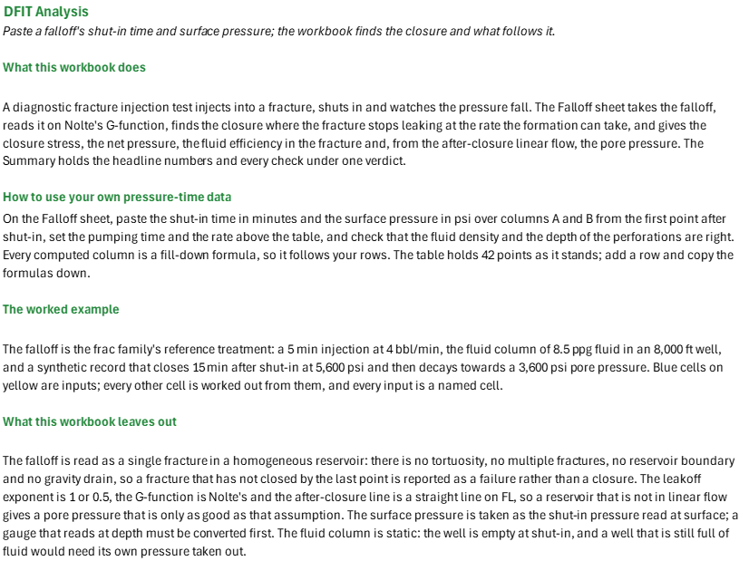
How to use it: Paste the shut-in time in minutes and the surface pressure in psi over columns A and B of the Falloff sheet, from the first point after shut-in, set the pumping time and the rate above the table, and check the fluid density and the depth of the perforations. Every computed column is a fill-down formula, so it follows your rows. A downhole gauge's record goes in column B with the fluid density set to zero. Smooth a noisy record before the derivative is read, set the tangent window past any early tortuosity or storage, and check the pick by eye on the G-function plot; your own closure G overrides it. The Summary holds the headline numbers and every check.
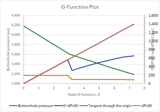
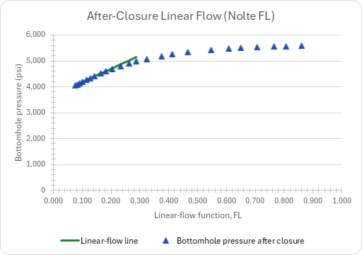
Method: The bottomhole pressure is the surface pressure plus the static column, which gives the bottomhole ISIP. With the dimensionless time dtD = dt/tp, Nolte's g is (4/3)[(1 + dtD)^1.5 - dtD^1.5] for alpha = 1 and G = (4/pi)(g - 4/3); dP/dG is a central difference and GdP/dG its product with G. While the fracture is open with normal leakoff the pressure falls on a straight line in G, so GdP/dG lies on a line through the origin; its slope is the least-squares fit over the tangent window of G, and closure is the first point past the window's start whose GdP/dG is more than the closure tolerance below that line. The closure time and stress are interpolated linearly in G. The net pressure is the bottomhole ISIP less the closure stress, and the efficiency is eta = Gc/(Gc + 4g0/pi). After closure, FL = (2/pi)*asin(sqrt(tc/t)) with tc = tp + dtc (Nolte 1997), and the least-squares line of pressure on the after-closure points with FL at most the largest FL fitted gives the pore pressure at FL = 0.
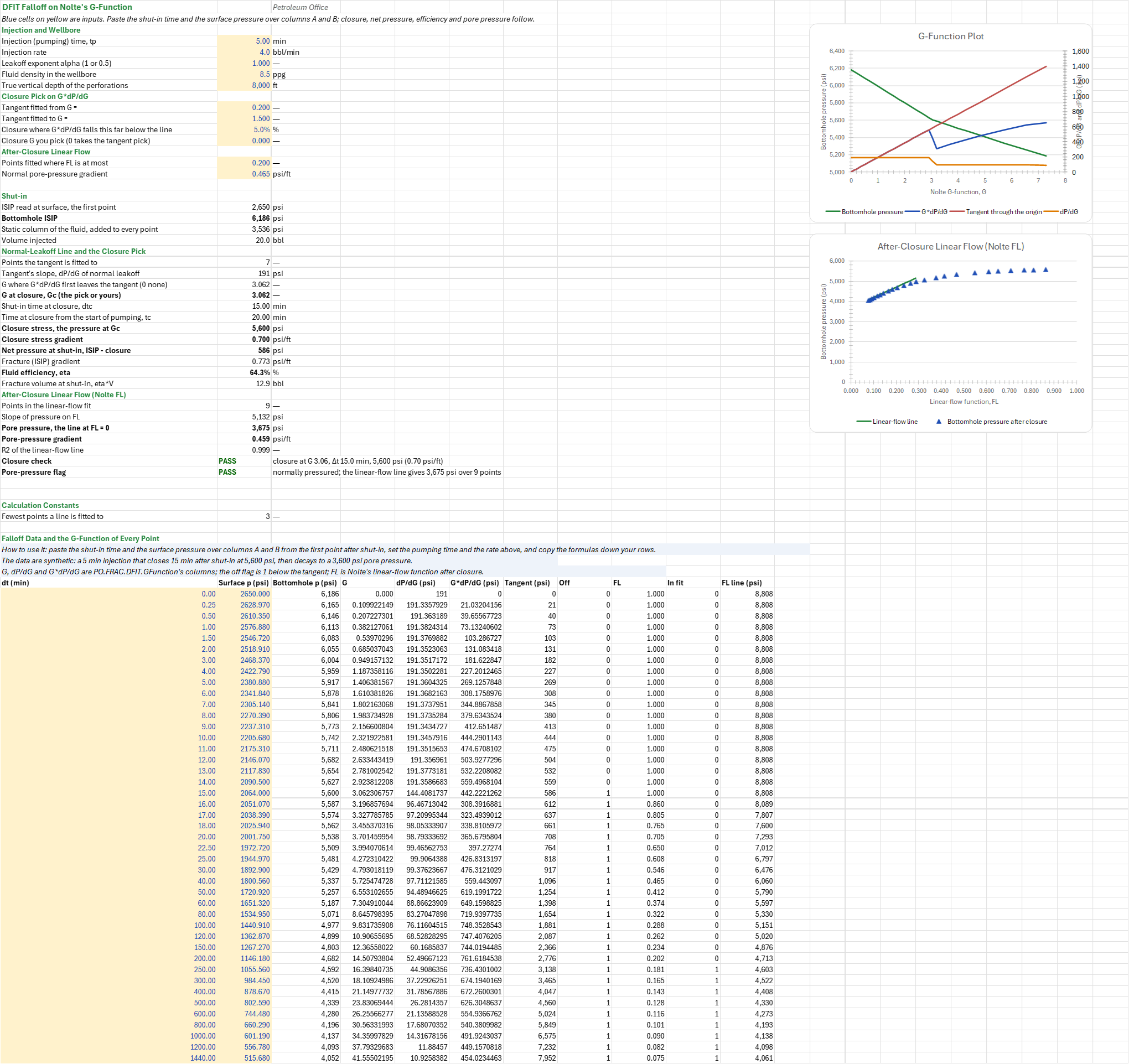
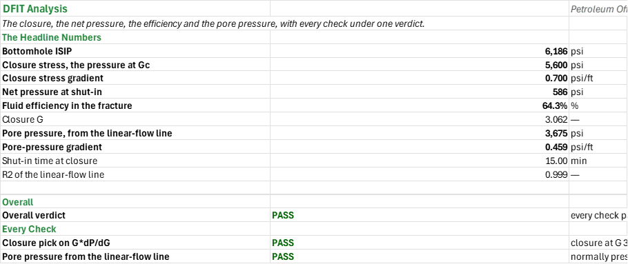
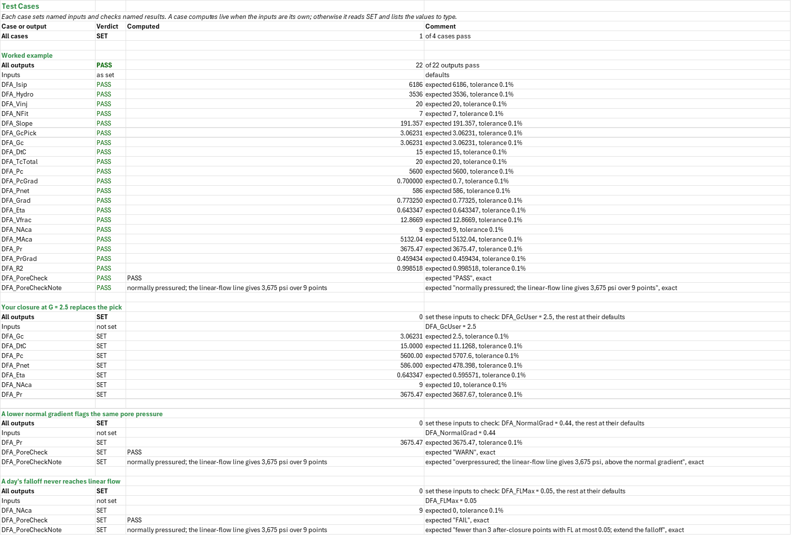
Example: The 3,536 psi column of 8.5 ppg fluid in an 8,000 ft well puts the bottomhole ISIP at 6,186 psi. Seven points from G = 0.21 to 1.41 fit a tangent of slope 191.36 psi, and the first point to fall more than 5 % below it is 15 min after shut-in, at G = 3.062: G*dP/dG is 442 there against the line's 586. Closure is at 5,600 psi, 0.700 psi/ft, and the net pressure at shut-in is 586 psi. The efficiency is 64.3 %, so 12.9 of the 20 bbl were still in the fracture at shut-in. Nine after-closure points have FL at most 0.2; their line has a slope of 5,132 psi and an R2 of 0.9985, and meets FL = 0 at 3,675 psi, 0.459 psi/ft: normally pressured. The intercept reads 75 psi above the model's 3,600 psi, because a day's falloff has not reached pure linear flow.
Validity
The G-function's assumptions: a single planar fracture, Carter leakoff, a constant injection rate and a fracture area that stops growing at shut-in. Pressure-dependent leakoff (a hump above the tangent), height recession or transverse storage (a belly below it) and tip extension (a rising G*dP/dG at a steeper line) each change the curve, and the pick then needs your judgement, which is what your own closure G on the Falloff sheet is for. The pick is late by up to one point, because the central difference at the first post-closure point mixes both slopes, so space the points closely around the expected closure. FL reaches pore pressure only once true linear flow is established, which in tight rock can take days, and before that the intercept reads high. The workbook does not analyse radial after-closure flow (FR, giving kh) or plot the sqrt(t) and log-log diagnostics. Spurt loss is left out of the efficiency.
References
- Nolte, K.G. (1979). "Determination of Fracture Parameters from Fracturing Pressure Decline." SPE 8341.
- Nolte, K.G. (1986). "A General Analysis of Fracturing Pressure Decline With Application to Three Models." SPE Formation Evaluation 1(6), 571-583.
- Nolte, K.G. (1997). "Background for After-Closure Analysis of Fracture Calibration Tests." SPE 39407.
- Economides, M.J. and Nolte, K.G. (eds.) (2000). Reservoir Stimulation, 3rd ed. Wiley, ch. 9.
Inputs
| Input | Unit | Default | Name |
|---|---|---|---|
| Injection (pumping) time, tp | min | 5 | DFA_Tp |
| Injection rate | bbl/min | 4 | DFA_Q |
| Leakoff exponent alpha (1 or 0.5) | - | 1 | DFA_Alpha |
| Fluid density in the wellbore | ppg | 8.5 | DFA_RhoFluid |
| True vertical depth of the perforations | ft | 8000 | DFA_Tvd |
| Tangent fitted from G =, to G = | - | 0.2, 1.5 | DFA_GLo, DFA_GHi |
| Closure where G*dP/dG falls this far below the line | fraction | 0.05 | DFA_Tol |
| Closure G you pick (0 takes the tangent pick) | - | 0 | DFA_GcUser |
| Points fitted where FL is at most | - | 0.2 | DFA_FLMax |
| Normal pore-pressure gradient | psi/ft | 0.465 | DFA_NormalGrad |
| Falloff data: shut-in time and surface pressure, 43 points | min, psi | see the sheet | DFA_Data |
Sheets
Guide— what the workbook does, how to use your own pressure-time data, the worked example and what the workbook leaves out.Falloff— the inputs, the shut-in, the normal-leakoff line and the closure pick, the after-closure linear flow, and the falloff table with the G-function of every point; two charts, the G-function plot (the bottomhole pressure, G*dP/dG, the tangent through the origin and dP/dG) and the after-closure plot (the linear-flow line and the pressure).Summary— the headline numbers (ISIP, closure stress and gradient, net pressure, efficiency, closure G, pore pressure and gradient, closure time, R2) and every check under one verdict.Test Cases— the worked example and other cases, with expected and computed results.
Functions used
Names (60)
| Name | Refers to | Comment |
|---|---|---|
PO.FRAC.DFIT.EfficiencyLAMBDA |
=LAMBDA(Gc, alpha, IF(AND(alpha<>1, alpha<>0.5), NA(), IF(Gc<0, NA(), Gc/(Gc+4/PI()*IF(alpha=1, 4/3, PI()/2))))) |
Fracturing fluid efficiency from the G-function at closure (Nolte material balance): η = Gc/(Gc + 4·g0/π), Gc/(2 + Gc) for alpha 0.5 and Gc/(Gc + 16/(3π)) for alpha 1. |
PO.FRAC.DFIT.GFunctionLAMBDA |
=LAMBDA(dt, tp, p, alpha, output, IF(OR(tp<=0, AND(alpha<>1, alpha<>0.5)), NA(), LET(td, dt/tp, gn, IF(alpha=1, 4/3*((1+td)^1.5-td^1.5), (1+td)*ASIN(1/SQRT(1+td))+SQRT(td)), gz, IF(alpha=1, 4/3, PI()/2), bigg, 4/PI()*(gn-gz), cnt, ROWS(p), ix, SEQUENCE(cnt), jx, TRANSPOSE(ix), nxt, --(jx=ix+(ix<cnt)), prv, --(jx=ix-(ix>1)), dpdg, -(MMULT(nxt, p)-MMULT(prv, p))/(MMULT(nxt, bigg)-MMULT(prv, bigg)), sel, IF(output="dtD", 1, IF(output="gNolte", 2, IF(output="G", 3, IF(output="dPdG", 4, IF(output="GdPdG", 5, 0))))), IF(sel=0, NA(), CHOOSE(sel, td, gn, bigg, dpdg, bigg*dpdg))))) |
Nolte G-function of a fracture falloff for leakoff exponent alpha 1 or 0.5; output column "dtD", "gNolte" g(ΔtD), "G", "dPdG" (−dp/dG) or "GdPdG" (G·dP/dG), central differences. |
PO.FRAC.Eval.ISIPLAMBDA |
=LAMBDA(isip_surf, rho_fluid, tvd, closure, output, IF(OR(rho_fluid<0, tvd<=0), NA(), LET(isip_bh, isip_surf+0.052*rho_fluid*tvd, IF(output="ISIP", isip_bh, IF(output="Pnet", isip_bh-closure, IF(output="Gradient", isip_bh/tvd, NA())))))) |
Instantaneous shut-in pressure at the fracture from the surface ISIP plus the static column 0.052·ρ·TVD; output "ISIP" (psi), "Pnet" (ISIP − closure, psi) or "Gradient" (psi/ft). |
DFA_Alpha |
Falloff!$B$6 |
|
DFA_Analysis |
Falloff!$C$54:$K$96 |
|
DFA_ClosureCheck |
Falloff!$B$42 |
|
DFA_ClosureCheckNote |
Falloff!$C$42 |
|
DFA_Data |
Falloff!$A$54:$B$96 |
|
DFA_DtC |
Falloff!$B$28 |
|
DFA_Eta |
Falloff!$B$34 |
|
DFA_FLMax |
Falloff!$B$15 |
|
DFA_GHi |
Falloff!$B$11 |
|
DFA_GLo |
Falloff!$B$10 |
|
DFA_GPlot |
Falloff!$C$54:$G$82 |
|
DFA_Gc |
Falloff!$B$27 |
|
DFA_GcPick |
Falloff!$B$26 |
|
DFA_GcUser |
Falloff!$B$13 |
|
DFA_Grad |
Falloff!$B$33 |
|
DFA_Hydro |
Falloff!$B$21 |
|
DFA_Inputs |
Falloff!$B$4:$B$16 |
|
DFA_Isip |
Falloff!$B$20 |
|
DFA_IsipSurf |
Falloff!$B$19 |
|
DFA_MAca |
Falloff!$B$38 |
|
DFA_NAca |
Falloff!$B$37 |
|
DFA_NFit |
Falloff!$B$24 |
|
DFA_NormalGrad |
Falloff!$B$16 |
|
DFA_Pc |
Falloff!$B$30 |
|
DFA_PcGrad |
Falloff!$B$31 |
|
DFA_Pnet |
Falloff!$B$32 |
|
DFA_PoreCheck |
Falloff!$B$43 |
|
DFA_PoreCheckNote |
Falloff!$C$43 |
|
DFA_Pr |
Falloff!$B$39 |
|
DFA_PrGrad |
Falloff!$B$40 |
|
DFA_Q |
Falloff!$B$5 |
|
DFA_R2 |
Falloff!$B$41 |
|
DFA_Results |
Falloff!$B$19:$B$43 |
|
DFA_RhoFluid |
Falloff!$B$7 |
|
DFA_Slope |
Falloff!$B$25 |
|
DFA_TcTotal |
Falloff!$B$29 |
|
DFA_Tol |
Falloff!$B$12 |
|
DFA_Tp |
Falloff!$B$4 |
|
DFA_Tvd |
Falloff!$B$8 |
|
DFA_Vfrac |
Falloff!$B$35 |
|
DFA_Vinj |
Falloff!$B$22 |
|
DFU_Checks |
Summary!$B$18:$B$19 |
|
DFU_DtC |
Summary!$B$12 |
|
DFU_Eta |
Summary!$B$8 |
|
DFU_Gc |
Summary!$B$9 |
|
DFU_Isip |
Summary!$B$4 |
|
DFU_Overall |
Summary!$B$16 |
|
DFU_OverallNote |
Summary!$C$16 |
|
DFU_Pc |
Summary!$B$5 |
|
DFU_PcGrad |
Summary!$B$6 |
|
DFU_Pnet |
Summary!$B$7 |
|
DFU_Pr |
Summary!$B$10 |
|
DFU_PrGrad |
Summary!$B$11 |
|
DFU_R2 |
Summary!$B$13 |
|
DFU_Results |
Summary!$B$4:$B$13 |
|
DFU_Verdict |
Summary!$B$16 |
|
DFU_VerdictNote |
Summary!$C$16 |
Details
| Opens in | Needs Microsoft 365 or Excel 2024: it uses functions Excel 2016 doesn't have, such as named LAMBDAs, which show #NAME? there. |
| File | DfitAnalysis.xlsx, 42 KB |
| Category | Reservoir |
| For agents and tools | Descriptor (.md) |