Waterflood Surveillance
Description
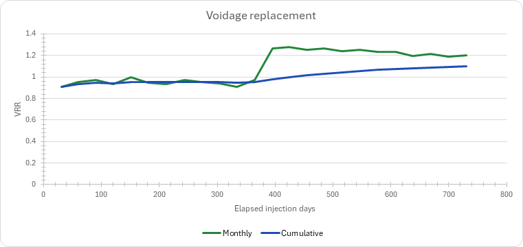
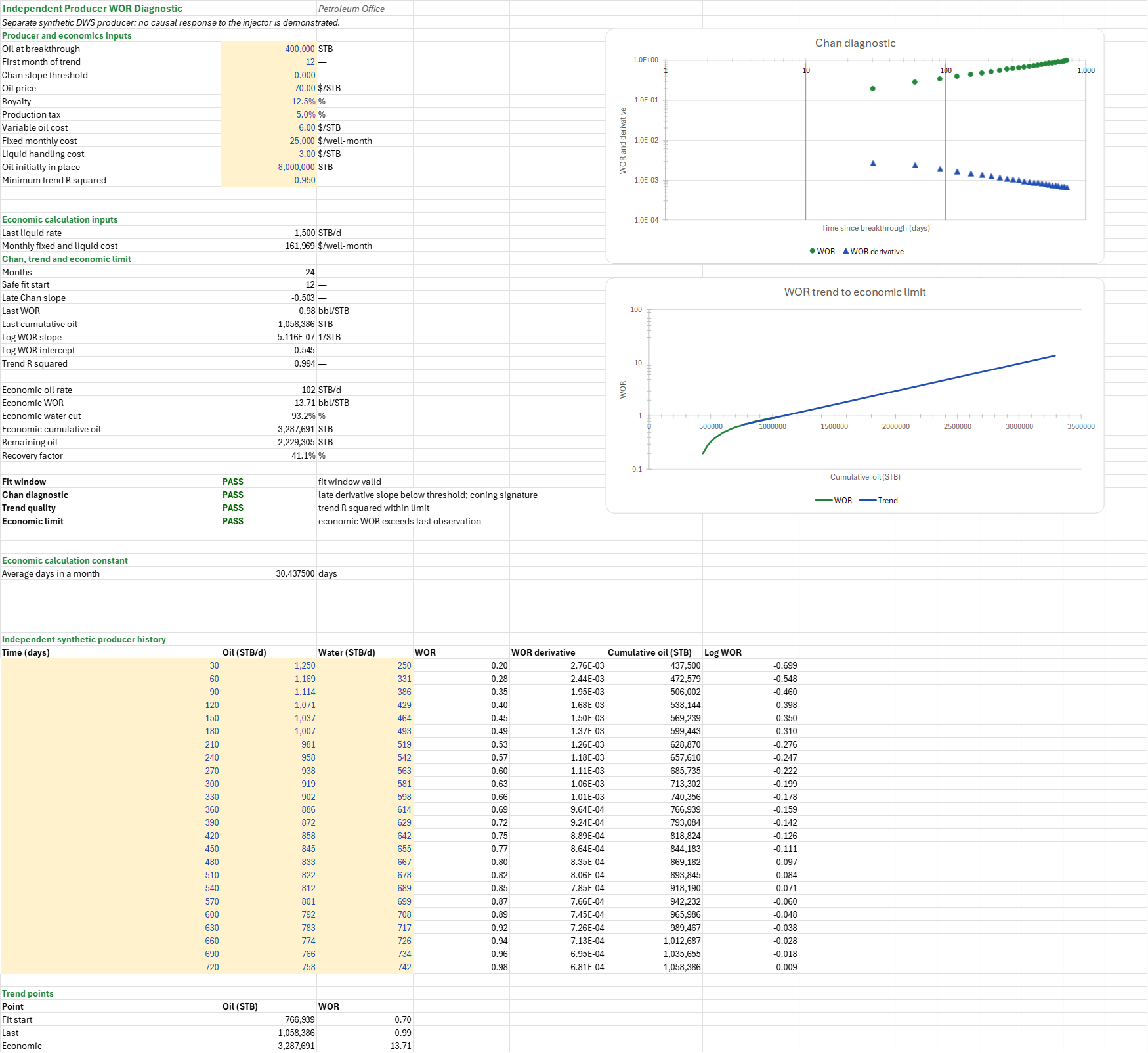
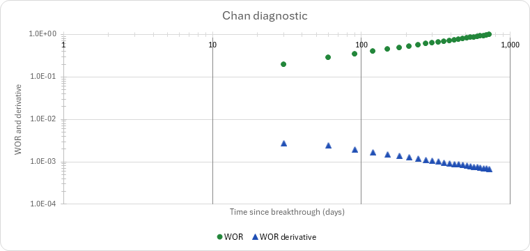
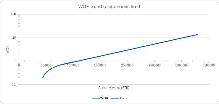
Is the injector plugging or fracturing, is the pattern's voidage being replaced, and what do a producer's water-oil ratio trends say about its water and its remaining oil? You enter an injector's monthly days, pressure and rate, the pattern's allocated production and injection, a producer's oil and water rates and an oil price and cost deck. You read off the Hall-plot slopes and skins, the monthly and cumulative voidage replacement ratio, the Chan diagnostic, and the oil recovered when the WOR trend reaches its economic limit. Field units.
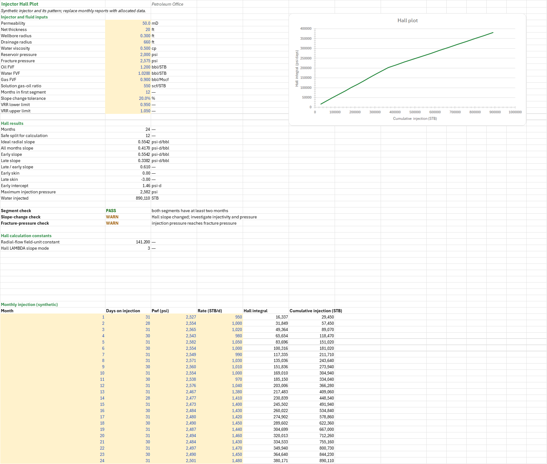
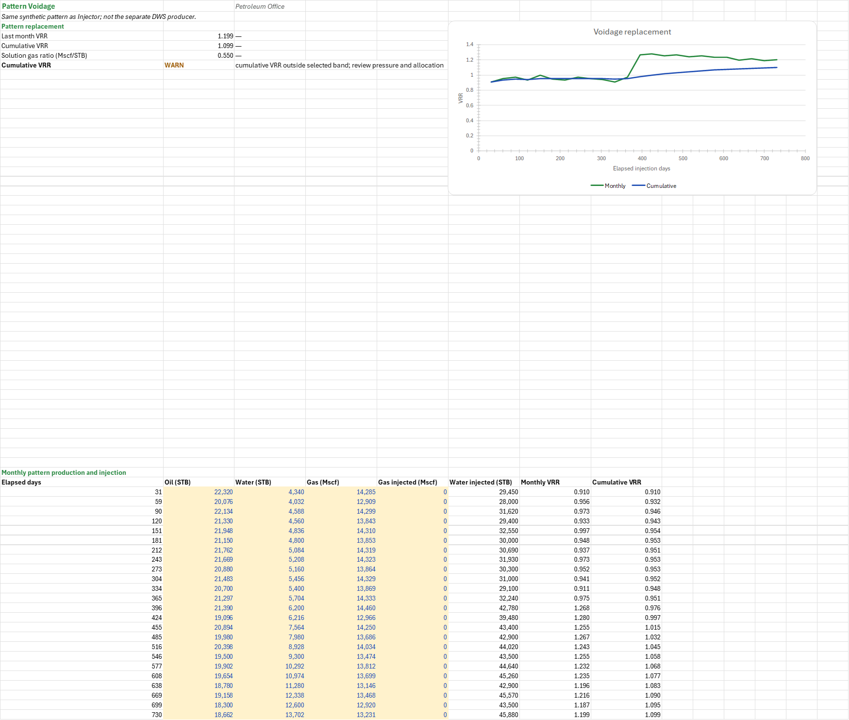
How to use it: Replace every synthetic monthly row with matched, quality-controlled field data: the injector's bottomhole injection pressure, days on injection and rate on the Injector sheet, and production allocated to the same pattern, with injected water and gas, on the Voidage sheet, using consistent fluid factors and units. Enter the producer's time from breakthrough and oil and water rates, and the economics, on the Producer sheet. Each table has 24 rows. Assess the pressure history and allocation before interpreting VRR, and for observational injector-producer comparisons match calendar dates and allocation first. The Summary places the observations side by side and lists every check; a failing check takes precedence over a warning. Needs Microsoft 365 or Excel 2024.
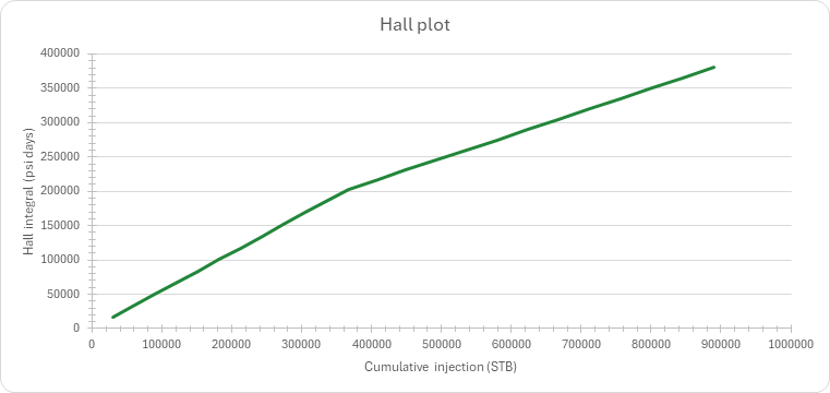
Method: The Hall integral is the cumulative pressure difference between the bottomhole injection pressure and the reservoir pressure times the injection days, plotted against cumulative water injected. Least-squares early and late slopes are fitted either side of the chosen split, and each slope gives a skin through steady radial flow between the wellbore and drainage radii. The monthly and cumulative VRR compare injected and produced reservoir volumes using the entered oil, water and gas formation volume factors and solution gas-oil ratio. The Producer sheet plots the WOR and its Chan derivative against time on log axes; it regresses log WOR against cumulative oil and extrapolates to an economic WOR at constant liquid rate and costs. The checks flag an invalid split or fit window, a slope change beyond the tolerance, pressure at the fracture limit, VRR outside the selected band, and diagnostic or trend concerns.
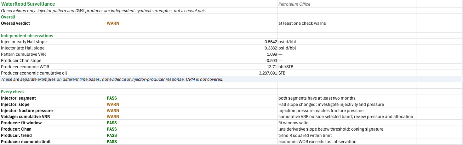
Example: Two independent synthetic examples. In the Hall pattern (24 monthly injection reports and allocated pattern production), the early and late slopes are 0.5542 and 0.3382 psi-day/STB and the cumulative VRR is 1.099; the slope, fracture-pressure and VRR checks warn at the default limits. In the separate 24-point DWS producer history, the Chan slope is -0.503 and the economic WOR trend reaches approximately 3.29 million STB. These examples are not a matched injector-producer pair and do not demonstrate a response between wells.
Validity
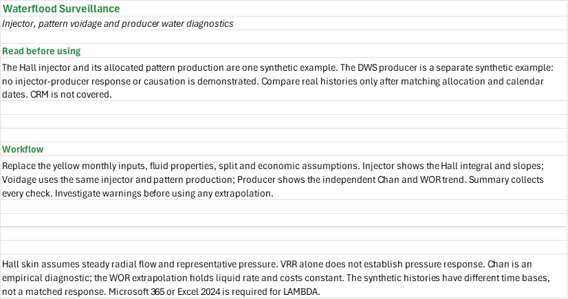
The injector and voidage example and the producer example are independent; no response or causal connection between them is demonstrated, and the Summary places them together only for comparison. Elapsed days on the Voidage chart sum the reported injection days, not necessarily calendar time. Hall skin assumes steady radial flow and a representative reservoir pressure. Chan signatures are empirical indicators, not proof of a water source; the WOR extrapolation assumes the trend, liquid rate and economics persist and can be unreliable outside the fitted interval. No time forecast is made. Capacitance-resistance (CRM) connectivity between injectors and producers is not covered.
References
- Hall, H.N. (1963). How to Analyse Waterflood Injection Well Performance. World Oil.
- Chan, K.S. (1995). Water Control Diagnostic Plots. SPE 30775.
Inputs
| Input | Unit | Default | Name |
|---|---|---|---|
| Permeability | mD | 50 | WSI_K |
| Net thickness | ft | 20 | WSI_H |
| Wellbore radius | ft | 0.3 | WSI_Rw |
| Drainage radius | ft | 660 | WSI_Re |
| Water viscosity | cp | 0.5 | WSI_Muw |
| Reservoir pressure | psi | 2000 | WSI_Pe |
| Fracture pressure | psi | 2575 | WSI_Pfrac |
| Oil FVF | rb/STB | 1.2 | WSI_Bo |
| Water FVF | rb/STB | 1.02 | WSI_Bw |
| Gas FVF | bbl/Mscf | 0.9 | WSI_Bg |
| Solution gas-oil ratio | scf/STB | 550 | WSI_Rs |
| Months in first segment | months | 12 | WSI_Split |
| Slope change tolerance | fraction | 0.2 | WSI_SlopeTol |
| VRR lower limit | fraction | 0.95 | WSI_VrrLo |
| VRR upper limit | fraction | 1.05 | WSI_VrrHi |
| Oil at breakthrough | STB | 400000 | WSP_Np0 |
| First month of trend | month | 12 | WSP_FitFrom |
| Chan slope threshold | fraction | 0 | WSP_SlopeConing |
| Oil price | $/STB | 70 | WSP_Price |
| Royalty | fraction | 0.125 | WSP_Royalty |
| Production tax | fraction | 0.05 | WSP_Tax |
| Variable oil cost | $/STB | 6 | WSP_Opex |
| Fixed monthly cost | $/month | 25000 | WSP_Fixed |
| Liquid handling cost | $/STB | 3 | WSP_Lift |
| Oil initially in place | STB | 8000000 | WSP_N |
| Minimum trend R squared | fraction | 0.95 | WSP_R2Min |
The Injector table holds editable injection days, pressure and rate; the Voidage table editable allocated oil, water, gas and injected gas; the Producer table editable time from breakthrough and oil and water rates. All have 24 rows.
Sheets
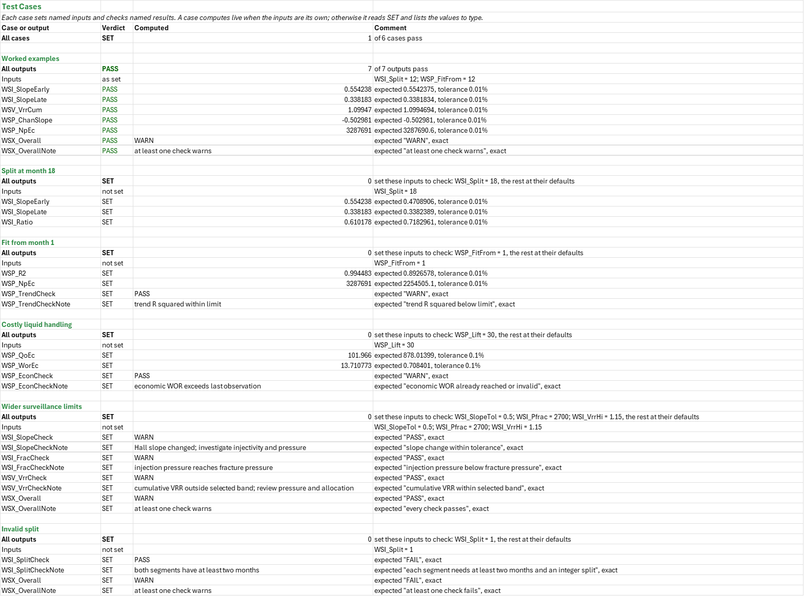
Guide— what to read before using the workbook, its scope and assumptions, and the workflow.Injector— the injector and fluid inputs, the monthly injection table, the Hall plot, and the early and late slopes with their skins.Voidage— the pattern's monthly production and injection, and its monthly and cumulative VRR against elapsed injection days.Producer— an independent producer's history, the Chan WOR and derivative plot, and the WOR trend against cumulative oil to the economic limit.Summary— the independent observations side by side and every check under one verdict; a failure overrides a warning.Test Cases— the worked example and other cases, with expected and computed results.
Functions used
Names (102)
| Name | Refers to | Comment |
|---|---|---|
PO.PE.Chan.WORDerivativeLAMBDA |
=LAMBDA(time, wor, at, LET(n, COUNT(time), k, MATCH(at, time, 0), k_lo, MAX(1, k-1), k_hi, MIN(n, k+1), t_k, INDEX(time, k), t_lo, INDEX(time, k_lo), t_hi, INDEX(time, k_hi), w_k, INDEX(wor, k), w_lo, INDEX(wor, k_lo), w_hi, INDEX(wor, k_hi), IF(k=1, (w_hi-w_k)/(t_hi-t_k), IF(k=n, (w_k-w_lo)/(t_k-t_lo), ((w_k-w_lo)/(t_k-t_lo)*(t_hi-t_k)+(w_hi-w_k)/(t_hi-t_k)*(t_k-t_lo))/(t_hi-t_lo))))) |
Chan (1995) WOR′: the time derivative of the water-oil ratio at one point of a production history, a three-point difference weighted by the neighbouring intervals, [1/time unit]. |
PO.RES.Reserves.EconLimitLAMBDA |
=LAMBDA(Price, Royalty, Tax, Opex, Fixed, LET(netback, Price*(1-Royalty)*(1-Tax)-Opex, IF(netback>0, Fixed/netback, NA()))) |
Economic-limit rate: fixed cost per period over the netback per unit after royalty, production tax and variable opex; #N/A if the netback is not positive |
PO.RES.Waterflood.HallLAMBDA |
=LAMBDA(dt, Pwf, Pe, Q, Mode, LET(hall, SCAN(0, (Pwf-Pe)*dt, LAMBDA(acc, v, acc+v)), wi, SCAN(0, Q*dt, LAMBDA(acc, v, acc+v)), IF(Mode=1, hall, IF(Mode=2, wi, IF(Mode=3, SLOPE(hall, wi), NA()))))) |
Hall plot of an injector: Mode 1 Hall integral, psi-d; 2 cumulative injection, bbl; 3 Hall slope, psi-d/bbl, by least squares |
PO.RES.Waterflood.VRRLAMBDA |
=LAMBDA(Np, Wp, Gp, Bo, Bw, Bg, Rs, Wi, Gi, Mode, LET(inj, Wi*Bw+Gi*Bg, wd, Np*Bo+(Gp-Np*Rs)*Bg+Wp*Bw, IF(Mode=1, inj/wd, IF(Mode=2, SCAN(0, inj, LAMBDA(acc, v, acc+v))/SCAN(0, wd, LAMBDA(acc, v, acc+v)), NA())))) |
Voidage replacement ratio in reservoir barrels, injected over withdrawn: Mode 1 per period, 2 cumulative |
WSI_Bg |
Injector!$B$13 |
Gas FVF, bbl/Mscf |
WSI_Bo |
Injector!$B$11 |
Oil FVF, bbl/STB |
WSI_Bw |
Injector!$B$12 |
Water FVF, bbl/STB |
WSI_Darcy |
Injector!$B$39 |
Radial-flow field-unit constant |
WSI_FracCheck |
Injector!$B$36 |
Fracture-pressure check verdict |
WSI_FracCheckNote |
Injector!$C$36 |
Fracture-pressure check comment |
WSI_H |
Injector!$B$5 |
Net thickness, ft |
WSI_History |
Injector!$A$51:$F$74 |
Month, Days on injection, Pwf (psi), Rate (STB/d), Hall integral, Cumulative injection (STB) |
WSI_Icpt |
Injector!$B$30 |
Early intercept, psi·d |
WSI_Ideal |
Injector!$B$23 |
Ideal radial slope, psi·d/bbl |
WSI_Inputs |
Injector!$B$4:$B$18 |
Injector rock, fluids, pressures, segment split and surveillance limits |
WSI_K |
Injector!$B$4 |
Permeability, mD |
WSI_ModeSlope |
Injector!$B$40 |
Hall LAMBDA slope mode |
WSI_Muw |
Injector!$B$8 |
Water viscosity, cp |
WSI_N |
Injector!$B$21 |
Months |
WSI_Pe |
Injector!$B$9 |
Reservoir pressure, psi |
WSI_Pfrac |
Injector!$B$10 |
Fracture pressure, psi |
WSI_Pwf |
Injector!$C$51:$C$74 |
Injection pressure |
WSI_PwfMax |
Injector!$B$31 |
Maximum injection pressure, psi |
WSI_Q |
Injector!$D$51:$D$74 |
Injection rate |
WSI_Ratio |
Injector!$B$27 |
Late / early slope |
WSI_Re |
Injector!$B$7 |
Drainage radius, ft |
WSI_Results |
Injector!$B$21:$B$32 |
Hall slopes, skins, pressure and cumulative injection |
WSI_Rs |
Injector!$B$14 |
Solution gas-oil ratio, scf/STB |
WSI_Rw |
Injector!$B$6 |
Wellbore radius, ft |
WSI_SafeSplit |
Injector!$B$22 |
Safe split for calculation |
WSI_SkinEarly |
Injector!$B$28 |
Early skin |
WSI_SkinLate |
Injector!$B$29 |
Late skin |
WSI_SlopeAll |
Injector!$B$24 |
All months slope, psi·d/bbl |
WSI_SlopeCheck |
Injector!$B$35 |
Slope-change check verdict |
WSI_SlopeCheckNote |
Injector!$C$35 |
Slope-change check comment |
WSI_SlopeEarly |
Injector!$B$25 |
Early slope, psi·d/bbl |
WSI_SlopeLate |
Injector!$B$26 |
Late slope, psi·d/bbl |
WSI_SlopeTol |
Injector!$B$16 |
Slope change tolerance, % |
WSI_Split |
Injector!$B$15 |
Months in first segment |
WSI_SplitCheck |
Injector!$B$34 |
Segment check verdict |
WSI_SplitCheckNote |
Injector!$C$34 |
Segment check comment |
WSI_VrrHi |
Injector!$B$18 |
VRR upper limit |
WSI_VrrLo |
Injector!$B$17 |
VRR lower limit |
WSI_Wi |
Injector!$B$32 |
Water injected, STB |
WSI_dt |
Injector!$B$51:$B$74 |
Days on injection |
WSP_A |
Producer!$B$27 |
Log WOR intercept |
WSP_B |
Producer!$B$26 |
Log WOR slope, 1/STB |
WSP_ChanCheck |
Producer!$B$38 |
Chan diagnostic verdict |
WSP_ChanCheckNote |
Producer!$C$38 |
Chan diagnostic comment |
WSP_ChanSlope |
Producer!$B$23 |
Late Chan slope |
WSP_DaysPerMonth |
Producer!$B$44 |
Average days in a month, days |
WSP_EconCheck |
Producer!$B$40 |
Economic limit verdict |
WSP_EconCheckNote |
Producer!$C$40 |
Economic limit comment |
WSP_FitFrom |
Producer!$B$5 |
First month of trend |
WSP_Fixed |
Producer!$B$11 |
Fixed monthly cost, $/well-month |
WSP_FwEc |
Producer!$B$32 |
Economic water cut, % |
WSP_History |
Producer!$A$51:$G$74 |
Time (days), Oil (STB/d), Water (STB/d), WOR, WOR derivative, Cumulative oil (STB), Log WOR |
WSP_Inputs |
Producer!$B$4:$B$14 |
Producer breakthrough, trend window, economics and recovery inputs |
WSP_Lift |
Producer!$B$12 |
Liquid handling cost, $/STB |
WSP_MonthlyCost |
Producer!$B$19 |
Monthly fixed and liquid cost, $/well-month |
WSP_Months |
Producer!$B$21 |
Months |
WSP_N |
Producer!$B$13 |
Oil initially in place, STB |
WSP_Np0 |
Producer!$B$4 |
Oil at breakthrough, STB |
WSP_NpEc |
Producer!$B$33 |
Economic cumulative oil, STB |
WSP_NpLast |
Producer!$B$25 |
Last cumulative oil, STB |
WSP_Opex |
Producer!$B$10 |
Variable oil cost, $/STB |
WSP_Price |
Producer!$B$7 |
Oil price, $/STB |
WSP_QL |
Producer!$B$18 |
Last liquid rate, STB/d |
WSP_QoEc |
Producer!$B$30 |
Economic oil rate, STB/d |
WSP_R2 |
Producer!$B$28 |
Trend R squared |
WSP_R2Min |
Producer!$B$14 |
Minimum trend R squared |
WSP_RF |
Producer!$B$35 |
Recovery factor, % |
WSP_Rem |
Producer!$B$34 |
Remaining oil, STB |
WSP_Results |
Producer!$B$21:$B$35 |
Chan diagnostic, trend and economic recovery results |
WSP_Royalty |
Producer!$B$8 |
Royalty, % |
WSP_SafeFit |
Producer!$B$22 |
Safe fit start |
WSP_SlopeConing |
Producer!$B$6 |
Chan slope threshold |
WSP_Tax |
Producer!$B$9 |
Production tax, % |
WSP_Trend |
Producer!$A$78:$C$80 |
Point, Oil (STB), WOR |
WSP_TrendCheck |
Producer!$B$39 |
Trend quality verdict |
WSP_TrendCheckNote |
Producer!$C$39 |
Trend quality comment |
WSP_WindowCheck |
Producer!$B$37 |
Fit window verdict |
WSP_WindowCheckNote |
Producer!$C$37 |
Fit window comment |
WSP_WorEc |
Producer!$B$31 |
Economic WOR, bbl/STB |
WSP_WorLast |
Producer!$B$24 |
Last WOR, bbl/STB |
WSV_History |
Voidage!$A$51:$H$74 |
Elapsed days, Oil (STB), Water (STB), Gas (Mscf), Gas injected (Mscf), Water injected (STB), Monthly VRR, Cumulative VRR |
WSV_Results |
Voidage!$B$4:$B$6 |
Monthly and cumulative replacement ratios and converted solution gas ratio |
WSV_RsMscf |
Voidage!$B$6 |
Solution gas ratio (Mscf/STB) |
WSV_VrrCheck |
Voidage!$B$7 |
Cumulative VRR verdict |
WSV_VrrCheckNote |
Voidage!$C$7 |
Cumulative VRR comment |
WSV_VrrCum |
Voidage!$B$5 |
Cumulative VRR |
WSV_VrrLast |
Voidage!$B$4 |
Last month VRR |
WSX_ChanSlope |
Summary!$B$10 |
Producer Chan slope |
WSX_Checks |
Summary!$B$16:$B$23 |
All component verdicts |
WSX_NpEc |
Summary!$B$12 |
Producer economic cumulative oil, STB |
WSX_Overall |
Summary!$B$4 |
Overall verdict verdict |
WSX_OverallNote |
Summary!$C$4 |
Overall verdict comment |
WSX_Results |
Summary!$B$7:$B$12 |
Injector, pattern and independent producer headlines |
WSX_SlopeEarly |
Summary!$B$7 |
Injector early Hall slope, psi·d/bbl |
WSX_SlopeLate |
Summary!$B$8 |
Injector late Hall slope, psi·d/bbl |
WSX_VrrCum |
Summary!$B$9 |
Pattern cumulative VRR |
WSX_WorEc |
Summary!$B$11 |
Producer economic WOR, bbl/STB |
Details
| Opens in | Needs Microsoft 365 or Excel 2024: it uses functions Excel 2016 doesn't have, such as named LAMBDAs, which show #NAME? there. |
| File | WaterfloodSurveillance.xlsx, 56 KB |
| Category | Reservoir |
| For agents and tools | Descriptor (.md) |