Waterflood Design
Description
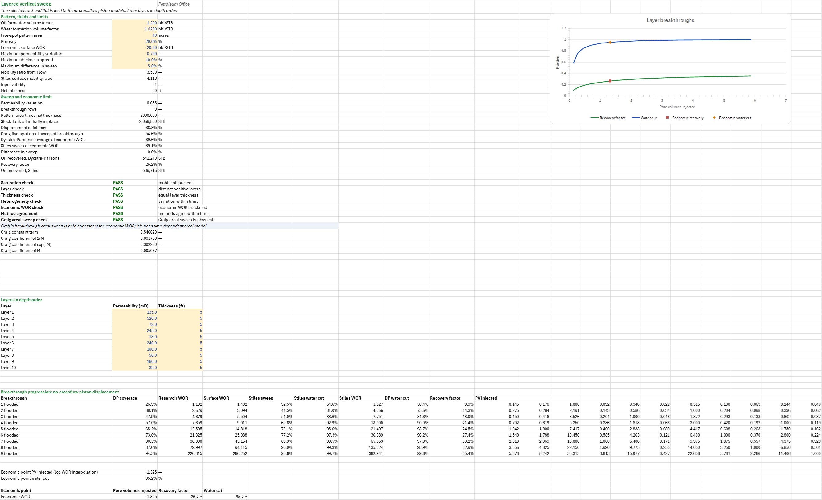
How much oil will a waterflood in a layered five-spot recover by the time the water-oil ratio reaches its economic limit? You enter the SCAL points and endpoints, the oil and water viscosities, the layer permeabilities and thicknesses, the pattern and the economic WOR. You read off the Corey exponents, the fractional-flow shock and breakthrough, the Dykstra-Parsons and Stiles vertical sweep, and the oil recovered and recovery factor at the economic WOR. Field units.
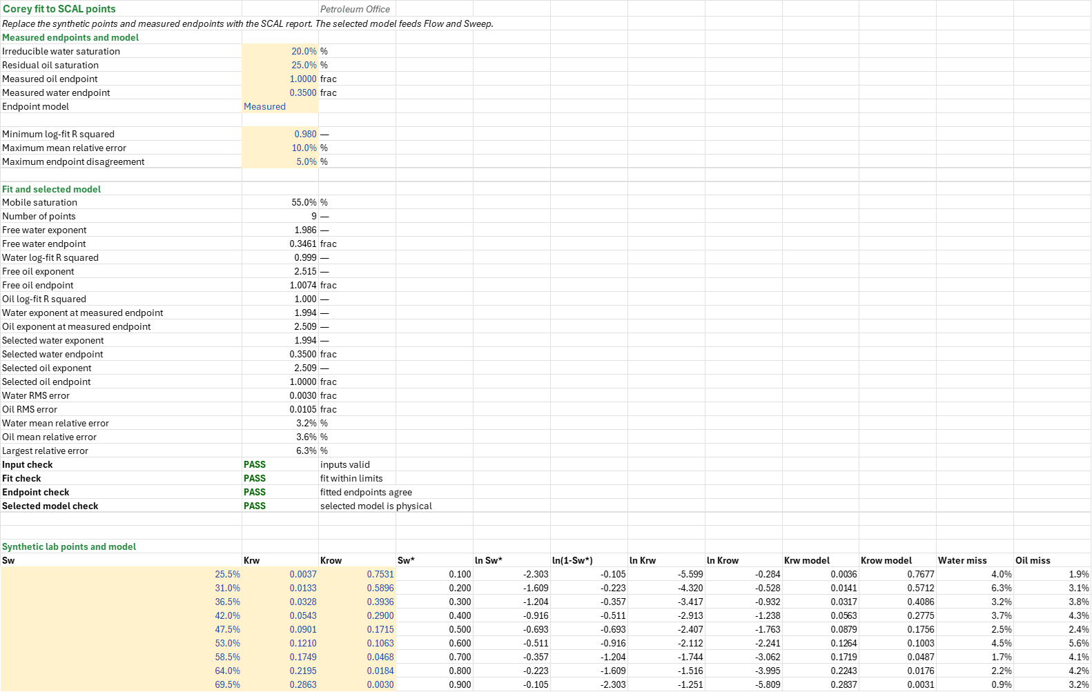
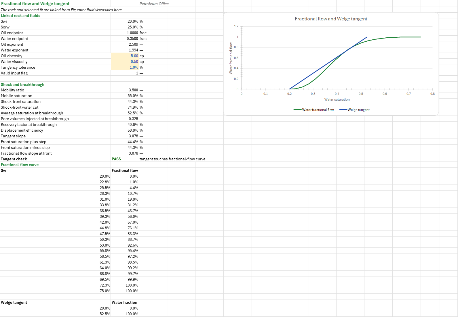
How to use it: Enter the SCAL relative-permeability points and the measured endpoints on the Fit sheet and choose whether the fit holds the measured endpoints or fits them freely. Enter the oil and water viscosities on the Flow sheet and check the Welge tangent touches the fractional-flow curve. Enter the layers in depth order, the pattern area, porosity, formation volume factors and the economic surface WOR on the Sweep sheet. The Summary links the results and every check. The examples are synthetic; replace the SCAL and layer tables with measured data.
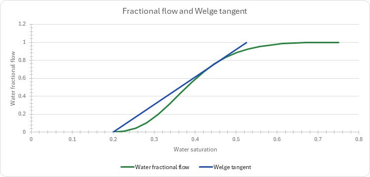
Method: The Fit sheet regresses ln krw against ln Sw* and ln kro against ln(1 − Sw*), with Sw* = (Sw − Swi)/(1 − Swi − Sorw) the normalised saturation, both freely and through the measured endpoints, for krw = krw° Sw*^nw and kro = kro° (1 − Sw*)^no; the default uses the measured endpoints. The Flow sheet applies the selected fit and viscosities to the Buckley-Leverett fractional flow fw = 1/(1 + (kro μw)/(krw μo)), finds the shock front by the Welge tangent, and gives the endpoint mobility ratio M = (krw°/μw)/(kro°/μo) and the displacement efficiency ED = (1 − Swi − Sorw)/(1 − Swi). The Sweep sheet applies Dykstra-Parsons and Stiles to the same endpoints, viscosities and saturations, interpolating between layer breakthroughs in log surface WOR. The oil in place is N = 7758 A h φ (1 − Swi)/Bo. Recovery is N × ED × vertical coverage × Craig's five-spot areal sweep at breakthrough, a correlation in M.
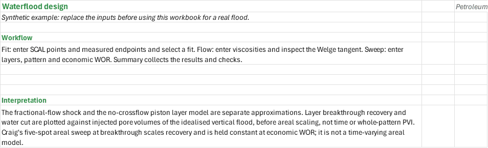
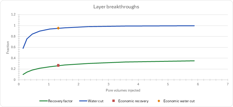
The layer-breakthrough PVI is the reservoir water injected over the pore volume of the idealised vertically layered flood (before areal scaling), not a whole-pattern material-balance PVI. For equal-thickness layers it is the mobile saturation times the mean of each layer's swept fraction plus the water injected after its breakthrough; for a layer already broken through, that is (M + 1)/2 × (k/k_break − 1). This is not a calendar-time forecast. The chart uses the same constant breakthrough areal sweep for every recovery point and for the economic point; it is an approximation, not a time-varying areal model.
Example: The shared synthetic SCAL rock has Swi 0.20, Sorw 0.25, and measured oil and water endpoints 1 and 0.35. With oil and water viscosities 5 and 0.5 cp, the endpoint mobility ratio is 3.5. Ten 5 ft layers in a 40-acre pattern (the classic Dykstra-Parsons example layers) on this rock, at an economic surface WOR of 20, give a vertical coverage of 0.6965 and an estimated recovery of 541,240 STB, 26.16% of the 2,068,800 STB initially in place. These are synthetic design inputs, not the layer example's original fluid and rock case.
Validity
Fractional flow is a one-dimensional Buckley-Leverett shock solution; Dykstra-Parsons and Stiles are separate no-crossflow, piston-displacement layer models, not a coupled fractional-flow forecast. Dykstra-Parsons and its PVI progression assume equal layer thickness and uniform porosity; Stiles accepts unequal thickness. Craig's areal sweep is a five-spot breakthrough correlation and need not hold for other geometries or at later times. An economic WOR outside the breakthrough range uses the nearest endpoint for recovery, injected PV and water cut, and warns; it is not extrapolated. Craig's raw areal sweep is checked for the physical interval from zero to one. A value outside that interval fails the check and sets the recovered oil and plotted recovery to zero; the zero is not a forecast. A free fit can imply an endpoint above one; this warns and stops the downstream calculations. Use measured SCAL, PVT and representative layer data, check mobility and geometrical applicability, and use simulation where crossflow, gravity or complex pattern geometry matters.
References
- Buckley, S.E. and Leverett, M.C. (1942). Mechanism of Fluid Displacement in Sands. Transactions of the AIME.
- Stiles, W.E. (1949). Use of Permeability Distribution in Water Flood Calculations. Transactions of the AIME.
- Dykstra, H. and Parsons, R.L. (1950). The Prediction of Oil Recovery by Waterflood.
- Craig, F.F. (1971). The Reservoir Engineering Aspects of Waterflooding. SPE Monograph 3.
Inputs
| Input | Unit | Default | Name |
|---|---|---|---|
| Irreducible water saturation | fraction | 0.20 | WGF_Swi |
| Residual oil saturation | fraction | 0.25 | WGF_Sorw |
| Measured oil endpoint | fraction | 1 | WGF_KroEnd |
| Measured water endpoint | fraction | 0.35 | WGF_KrwEnd |
| Endpoint model (Measured or Free) | text | Measured | WGF_Pick |
| Oil viscosity | cp | 5 | WGFLOW_MuO |
| Water viscosity | cp | 0.5 | WGFLOW_MuW |
| Oil formation volume factor | rb/STB | 1.2 | WGS_Bo |
| Water formation volume factor | rb/STB | 1.02 | WGS_Bw |
| Five-spot pattern area | acres | 40 | WGS_Area |
| Porosity | fraction | 0.2 | WGS_Phi |
| Economic surface WOR | STB/STB | 20 | WGS_WorEc |
The SCAL points on the Fit sheet and the layer permeabilities and thicknesses on the Sweep sheet are editable tables.
Sheets
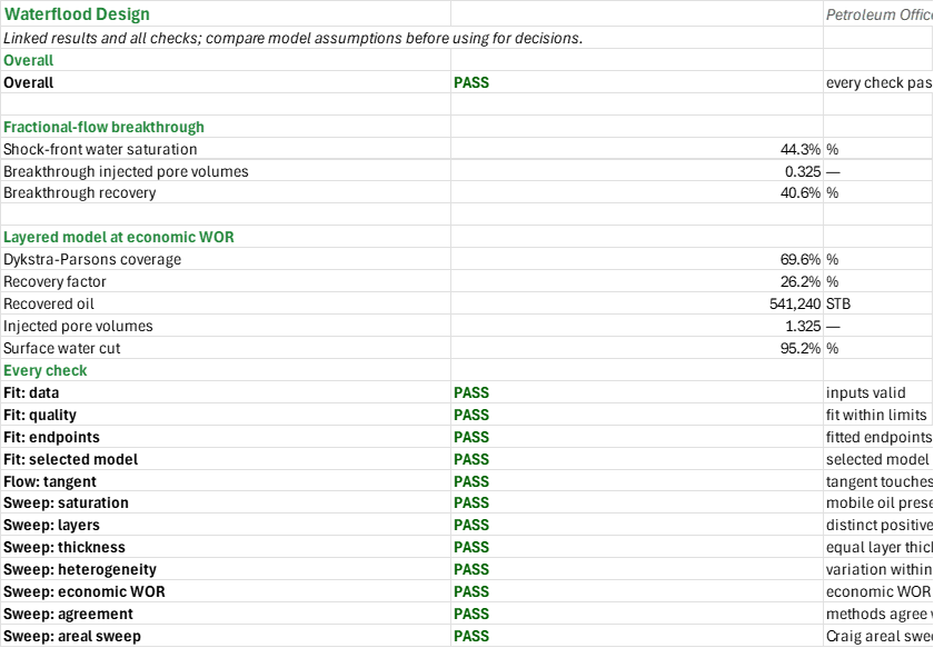
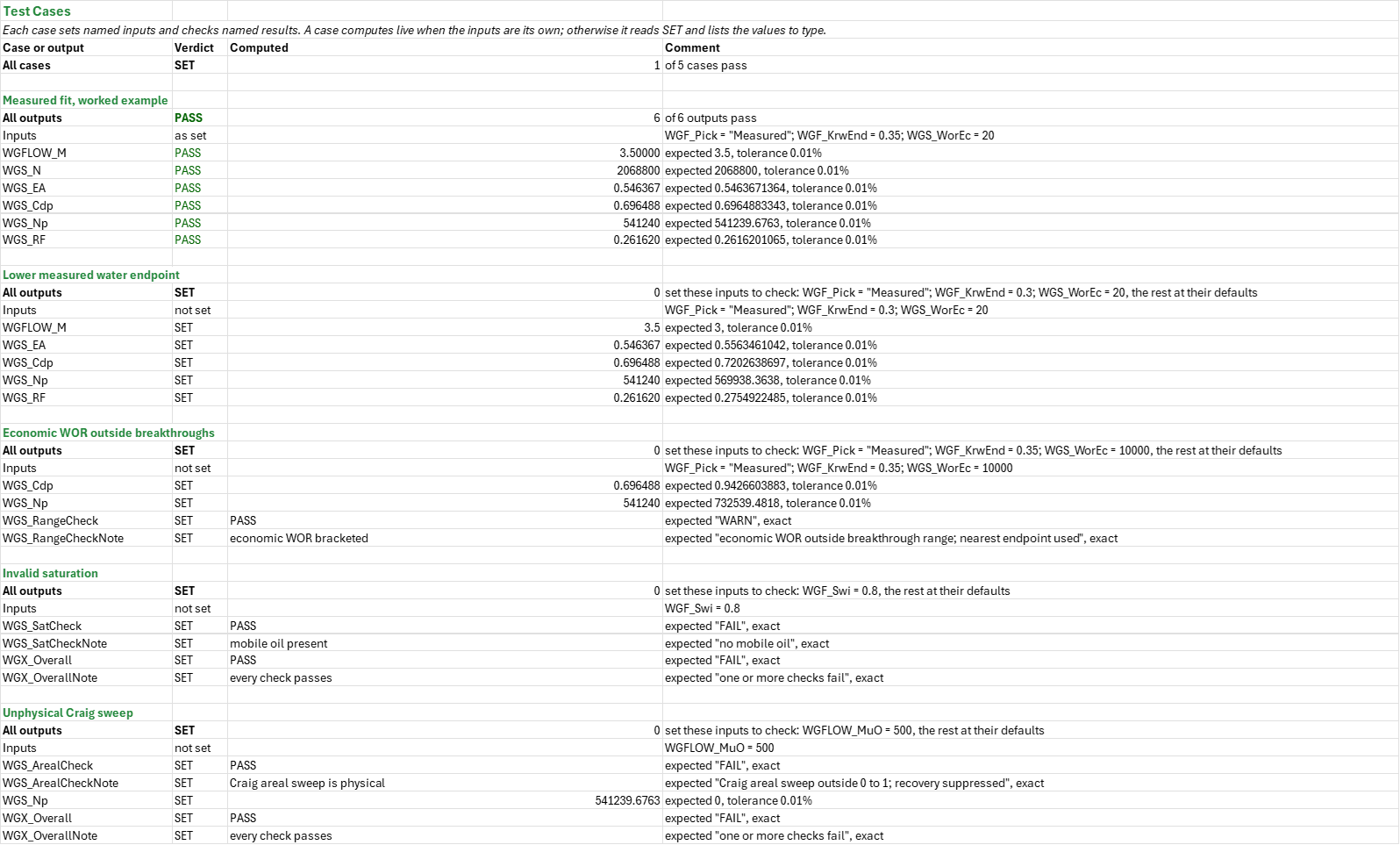
Guide— the workflow and how to read the separate models.Fit— the measured endpoints and the endpoint model; Corey exponents fitted freely and through the measured endpoints, the fit quality, the selected model, and the synthetic lab points against it.Flow— the rock and fit linked from Fit with the viscosities; the mobility ratio, shock-front saturation and water cut, the average saturation, pore volumes injected and recovery at breakthrough, the displacement efficiency, and the fractional-flow curve with its Welge tangent.Sweep— the pattern, fluids and layers; the permeability variation, oil in place, Craig's areal sweep, the Dykstra-Parsons coverage and Stiles sweep at the economic WOR, the oil recovered, and the breakthrough progression with recovery and water cut against injected pore volumes.Summary— the breakthrough and economic-WOR results linked from the sheets and every check under one verdict.Test Cases— the worked example and other cases, with expected and computed results.
Functions used
Names (140)
| Name | Refers to | Comment |
|---|---|---|
PO.RES.Vol.STOIIPLAMBDA |
=LAMBDA(GRV, NTG, Phi, Sw, Bo, 7758*GRV*NTG*Phi*(1-Sw)/Bo) |
Stock-tank oil initially in place, STB: 7758 x GRV (acre-ft) x NTG x porosity x (1 - Sw) / Bo (rb/STB). |
PO.RES.Waterflood.DykstraParsonsLAMBDA |
=LAMBDA(k, Mob, Mode, LET(n, ROWS(k), Vdp, 1-EXP(-STDEV.S(LN(k))), ks, SORT(k, , -1), kr, TRANSPOSE(ks), ratio, kr/ks, below, IF(ratio<1, ratio, 1), x, IF(ratio>=1, 1, IF(Mob=1, below, (Mob-SQRT(Mob^2+below*(1-Mob^2)))/(Mob-1))), ones, SEQUENCE(n, 1, 1, 0), cov, MMULT(x, ones)/n, wat, MMULT((ratio>=1)*kr, ones), oil, MMULT((ratio<1)*kr/(Mob+x*(1-Mob)), ones), open, oil>0, IF(Mode=1, Vdp, IF(Mode=2, FILTER(cov, open), IF(Mode=3, FILTER(wat/IF(open, oil, 1), open), NA()))))) |
Dykstra-Parsons layered waterflood: Mode 1 permeability variation V, 2 vertical coverage, 3 reservoir WOR, at each layer breakthrough |
PO.RES.Waterflood.FractionalFlowLAMBDA |
=LAMBDA(Sw, Swi, Sor, kro_end, krw_end, no, nw, mu_o, mu_w, output, LET(mob, 1-Swi-Sor, grid_a, SEQUENCE(399)/400, lw_a, krw_end*grid_a^nw/mu_w, ratio_a, lw_a/(lw_a+kro_end*(1-grid_a)^no/mu_o)/grid_a, idx_a, MATCH(MAX(ratio_a), ratio_a, 0), grid_b, (idx_a-1+SEQUENCE(400)/200)/400, lw_b, krw_end*grid_b^nw/mu_w, ratio_b, lw_b/(lw_b+kro_end*(1-grid_b)^no/mu_o)/grid_b, snf, INDEX(grid_b, MATCH(MAX(ratio_b), ratio_b, 0)), lwf, krw_end*snf^nw/mu_w, fwf, lwf/(lwf+kro_end*(1-snf)^no/mu_o), pv_bt, IF(mob>0, mob*snf/fwf, 0), sn, IF(mob>0, MIN(1, MAX(0, (Sw-Swi)/mob)), 0), lw, krw_end*sn^nw/mu_w, fw, lw/(lw+kro_end*(1-sn)^no/mu_o), IF(mob<=0, NA(), IF(output="fw", fw, IF(output="Swf", Swi+mob*snf, IF(output="fwf", fwf, IF(output="Swbar", Swi+pv_bt, IF(output="PVbt", pv_bt, NA())))))))) |
Buckley-Leverett fw on Corey curves and Welge's tangent from (Swi, 0); output "fw" (at Sw), "Swf" (shock front), "fwf", "Swbar" (mean Sw behind the front at breakthrough) or "PVbt" (PV injected by then). |
PO.RES.Waterflood.StilesLAMBDA |
=LAMBDA(k, h, A_wo, Mode, LET(f, (TRANSPOSE(k)>=k)*1, kh_cum, MMULT(f, k*h), h_cum, MMULT(f, h), kh_tot, SUM(k*h), h_tot, SUM(h), swept, (h_cum+(kh_tot-kh_cum)/k)/h_tot, fw, A_wo*kh_cum/(A_wo*kh_cum+kh_tot-kh_cum), IF(Mode=1, SORT(swept), IF(Mode=2, SORT(fw), NA())))) |
Stiles layered waterflood at each layer breakthrough, highest permeability first: Mode 1 fraction of the floodable volume swept, 2 surface water cut |
WGFLOW_Check |
Flow!$B$28 |
Tangent check verdict |
WGFLOW_CheckNote |
Flow!$C$28 |
Tangent check comment |
WGFLOW_Curve |
Flow!$A$31:$B$51 |
Fractional flow across the mobile range |
WGFLOW_DfDs |
Flow!$B$27 |
Fractional flow slope at front |
WGFLOW_Ed |
Flow!$B$23 |
Displacement efficiency, % |
WGFLOW_Fwf |
Flow!$B$19 |
Shock-front water cut, % |
WGFLOW_Inputs |
Flow!$B$10:$B$12 |
Fluid viscosities and tangent tolerance |
WGFLOW_KroEnd |
Flow!$B$6 |
Oil endpoint, frac |
WGFLOW_KrwEnd |
Flow!$B$7 |
Water endpoint, frac |
WGFLOW_M |
Flow!$B$16 |
Mobility ratio |
WGFLOW_Mobile |
Flow!$B$17 |
Mobile saturation, % |
WGFLOW_MuO |
Flow!$B$10 |
Oil viscosity, cp |
WGFLOW_MuW |
Flow!$B$11 |
Water viscosity, cp |
WGFLOW_No |
Flow!$B$8 |
Oil exponent |
WGFLOW_Nw |
Flow!$B$9 |
Water exponent |
WGFLOW_PVbt |
Flow!$B$21 |
Pore volumes injected at breakthrough |
WGFLOW_RFbt |
Flow!$B$22 |
Recovery factor at breakthrough, % |
WGFLOW_Slope |
Flow!$B$24 |
Tangent slope |
WGFLOW_Sorw |
Flow!$B$5 |
Sorw, % |
WGFLOW_SwMinus |
Flow!$B$26 |
Front saturation minus step, % |
WGFLOW_SwPlus |
Flow!$B$25 |
Front saturation plus step, % |
WGFLOW_Swbar |
Flow!$B$20 |
Average saturation at breakthrough, % |
WGFLOW_Swf |
Flow!$B$18 |
Shock-front saturation, % |
WGFLOW_Swi |
Flow!$B$4 |
Swi, % |
WGFLOW_Tol |
Flow!$B$12 |
Tangency tolerance, % |
WGFLOW_Valid |
Flow!$B$13 |
Valid input flag |
WGF_AareMax |
Fit!$B$11 |
Maximum mean relative error, % |
WGF_AareO |
Fit!$B$32 |
Oil mean relative error, % |
WGF_AareW |
Fit!$B$31 |
Water mean relative error, % |
WGF_DataCheck |
Fit!$B$34 |
Input check verdict |
WGF_DataCheckNote |
Fit!$C$34 |
Input check comment |
WGF_EndCheck |
Fit!$B$36 |
Endpoint check verdict |
WGF_EndCheckNote |
Fit!$C$36 |
Endpoint check comment |
WGF_EndTol |
Fit!$B$12 |
Maximum endpoint disagreement, % |
WGF_FitCheck |
Fit!$B$35 |
Fit check verdict |
WGF_FitCheckNote |
Fit!$C$35 |
Fit check comment |
WGF_Inputs |
Fit!$B$4:$B$12 |
Measured endpoints, fit selection and fit-check limits |
WGF_KroEnd |
Fit!$B$6 |
Measured oil endpoint, frac |
WGF_KroFit |
Fit!$B$21 |
Free oil endpoint, frac |
WGF_KroMod |
Fit!$J$42:$J$50 |
KroMod |
WGF_Krow |
Fit!$C$42:$C$50 |
Krow |
WGF_Krw |
Fit!$B$42:$B$50 |
Krw |
WGF_KrwEnd |
Fit!$B$7 |
Measured water endpoint, frac |
WGF_KrwFit |
Fit!$B$18 |
Free water endpoint, frac |
WGF_KrwMod |
Fit!$I$42:$I$50 |
KrwMod |
WGF_Ln1S |
Fit!$F$42:$F$50 |
Ln1S |
WGF_LnKrow |
Fit!$H$42:$H$50 |
LnKrow |
WGF_LnKrw |
Fit!$G$42:$G$50 |
LnKrw |
WGF_LnS |
Fit!$E$42:$E$50 |
LnS |
WGF_MaxMiss |
Fit!$B$33 |
Largest relative error, % |
WGF_MissO |
Fit!$L$42:$L$50 |
MissO |
WGF_MissW |
Fit!$K$42:$K$50 |
MissW |
WGF_Mobile |
Fit!$B$15 |
Mobile saturation, % |
WGF_ModelCheck |
Fit!$B$37 |
Selected model check verdict |
WGF_ModelCheckNote |
Fit!$C$37 |
Selected model check comment |
WGF_NPts |
Fit!$B$16 |
Number of points |
WGF_No |
Fit!$B$20 |
Free oil exponent |
WGF_NoFix |
Fit!$B$24 |
Oil exponent at measured endpoint |
WGF_Nw |
Fit!$B$17 |
Free water exponent |
WGF_NwFix |
Fit!$B$23 |
Water exponent at measured endpoint |
WGF_Pick |
Fit!$B$8 |
Endpoint model |
WGF_Points |
Fit!$A$42:$L$50 |
Synthetic SCAL points, logarithms and model errors |
WGF_R2Min |
Fit!$B$10 |
Minimum log-fit R squared |
WGF_R2o |
Fit!$B$22 |
Oil log-fit R squared |
WGF_R2w |
Fit!$B$19 |
Water log-fit R squared |
WGF_RmseO |
Fit!$B$30 |
Oil RMS error, frac |
WGF_RmseW |
Fit!$B$29 |
Water RMS error, frac |
WGF_Sn |
Fit!$D$42:$D$50 |
Sn |
WGF_Sorw |
Fit!$B$5 |
Residual oil saturation, % |
WGF_Sw |
Fit!$A$42:$A$50 |
Sw |
WGF_Swi |
Fit!$B$4 |
Irreducible water saturation, % |
WGF_UseKro |
Fit!$B$28 |
Selected oil endpoint, frac |
WGF_UseKrw |
Fit!$B$26 |
Selected water endpoint, frac |
WGF_UseNo |
Fit!$B$27 |
Selected oil exponent |
WGF_UseNw |
Fit!$B$25 |
Selected water exponent |
WGS_A |
Sweep!$B$13 |
Stiles surface mobility ratio |
WGS_AgreeTol |
Sweep!$B$11 |
Maximum difference in sweep, % |
WGS_AgreementCheck |
Sweep!$B$35 |
Method agreement verdict |
WGS_AgreementCheckNote |
Sweep!$C$35 |
Method agreement comment |
WGS_Area |
Sweep!$B$6 |
Five-spot pattern area, acres |
WGS_ArealCheck |
Sweep!$B$36 |
Craig areal sweep check verdict |
WGS_ArealCheckNote |
Sweep!$C$36 |
Craig areal sweep check comment |
WGS_Bo |
Sweep!$B$4 |
Oil formation volume factor, bbl/STB |
WGS_Breakthroughs |
Sweep!$A$66:$J$74 |
Layer breakthroughs and modelled pore volumes injected |
WGS_Bt |
Sweep!$B$18 |
Breakthrough rows |
WGS_Bulk |
Sweep!$B$19 |
Pattern area times net thickness |
WGS_Bw |
Sweep!$B$5 |
Water formation volume factor, bbl/STB |
WGS_Cdp |
Sweep!$B$23 |
Dykstra-Parsons coverage at economic WOR, % |
WGS_EA |
Sweep!$B$22 |
Craig five-spot areal sweep at breakthrough, % |
WGS_ED |
Sweep!$B$21 |
Displacement efficiency, % |
WGS_EaA |
Sweep!$B$38 |
Craig constant term |
WGS_EaB |
Sweep!$B$39 |
Craig coefficient of 1/M |
WGS_EaC |
Sweep!$B$40 |
Craig coefficient of exp(-M) |
WGS_EaD |
Sweep!$B$41 |
Craig coefficient of M |
WGS_FwEc |
Sweep!$B$78 |
Economic point water cut, % |
WGS_Gap |
Sweep!$B$25 |
Difference in sweep, % |
WGS_HTol |
Sweep!$B$10 |
Maximum thickness spread, % |
WGS_HeterogeneityCheck |
Sweep!$B$33 |
Heterogeneity check verdict |
WGS_HeterogeneityCheckNote |
Sweep!$C$33 |
Heterogeneity check comment |
WGS_Hnet |
Sweep!$B$15 |
Net thickness, ft |
WGS_Inputs |
Sweep!$B$4:$B$11 |
Pattern, fluid factors, economic WOR and check limits |
WGS_LayerCheck |
Sweep!$B$31 |
Layer check verdict |
WGS_LayerCheckNote |
Sweep!$C$31 |
Layer check comment |
WGS_Layers |
Sweep!$A$51:$C$60 |
Synthetic layer permeability and thickness |
WGS_M |
Sweep!$B$12 |
Mobility ratio from Flow |
WGS_N |
Sweep!$B$20 |
Stock-tank oil initially in place, STB |
WGS_Np |
Sweep!$B$26 |
Oil recovered, Dykstra-Parsons, STB |
WGS_NpSt |
Sweep!$B$28 |
Oil recovered, Stiles, STB |
WGS_PVEc |
Sweep!$B$77 |
Economic point PV injected (log WOR interpolation) |
WGS_Phi |
Sweep!$B$7 |
Porosity, % |
WGS_RF |
Sweep!$B$27 |
Recovery factor, % |
WGS_RangeCheck |
Sweep!$B$34 |
Economic WOR check verdict |
WGS_RangeCheckNote |
Sweep!$C$34 |
Economic WOR check comment |
WGS_Rst |
Sweep!$B$24 |
Stiles sweep at economic WOR, % |
WGS_SatCheck |
Sweep!$B$30 |
Saturation check verdict |
WGS_SatCheckNote |
Sweep!$C$30 |
Saturation check comment |
WGS_ThicknessCheck |
Sweep!$B$32 |
Thickness check verdict |
WGS_ThicknessCheckNote |
Sweep!$C$32 |
Thickness check comment |
WGS_V |
Sweep!$B$17 |
Permeability variation |
WGS_VMax |
Sweep!$B$9 |
Maximum permeability variation |
WGS_Valid |
Sweep!$B$14 |
Input validity |
WGS_WorEc |
Sweep!$B$8 |
Economic surface WOR, bbl/STB |
WGS_h |
Sweep!$C$51:$C$60 |
Layer thickness |
WGS_k |
Sweep!$B$51:$B$60 |
Layer permeability |
WGX_Breakthrough_Results |
Summary!$B$7:$B$9 |
Fractional-flow breakthrough headlines |
WGX_Cdp |
Summary!$B$12 |
Dykstra-Parsons coverage, % |
WGX_Economic_Results |
Summary!$B$12:$B$16 |
Layered-model economic WOR headlines |
WGX_FwEc |
Summary!$B$16 |
Surface water cut, % |
WGX_Np |
Summary!$B$14 |
Recovered oil, STB |
WGX_Overall |
Summary!$B$4 |
Overall verdict |
WGX_OverallNote |
Summary!$C$4 |
Overall comment |
WGX_PVEc |
Summary!$B$15 |
Injected pore volumes |
WGX_PVbt |
Summary!$B$8 |
Breakthrough injected pore volumes |
WGX_RF |
Summary!$B$13 |
Recovery factor, % |
WGX_RFbt |
Summary!$B$9 |
Breakthrough recovery, % |
WGX_Swf |
Summary!$B$7 |
Shock-front water saturation, % |
Details
| Opens in | Needs Microsoft 365 or Excel 2024: it uses functions Excel 2016 doesn't have, such as named LAMBDAs, which show #NAME? there. |
| File | WaterfloodDesign.xlsx, 51 KB |
| Category | Reservoir |
| For agents and tools | Descriptor (.md) |