Buildup Interpretation
Description
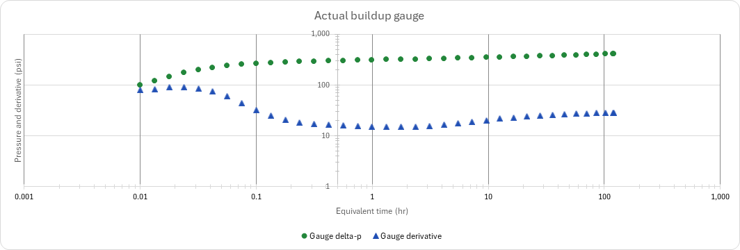
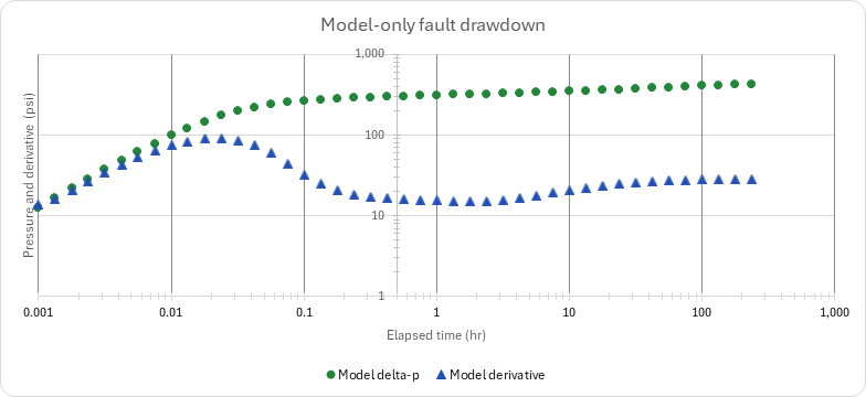
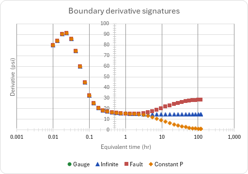
What permeability, skin and p-star does this oil buildup give, and does it see a boundary? You enter the rate before shut-in, the cumulative oil, the rock and fluid properties and the flowing pressure at shut-in, and paste the gauge's shut-in times and pressures. The Bourdet derivative picks the radial-flow (IARF) window, a Horner line through it gives k, skin and p-star, and the late slope reads a sealing fault or a constant-pressure boundary and the distance to a fault. Field units; time in hours.
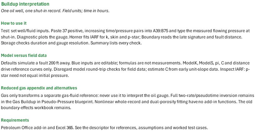
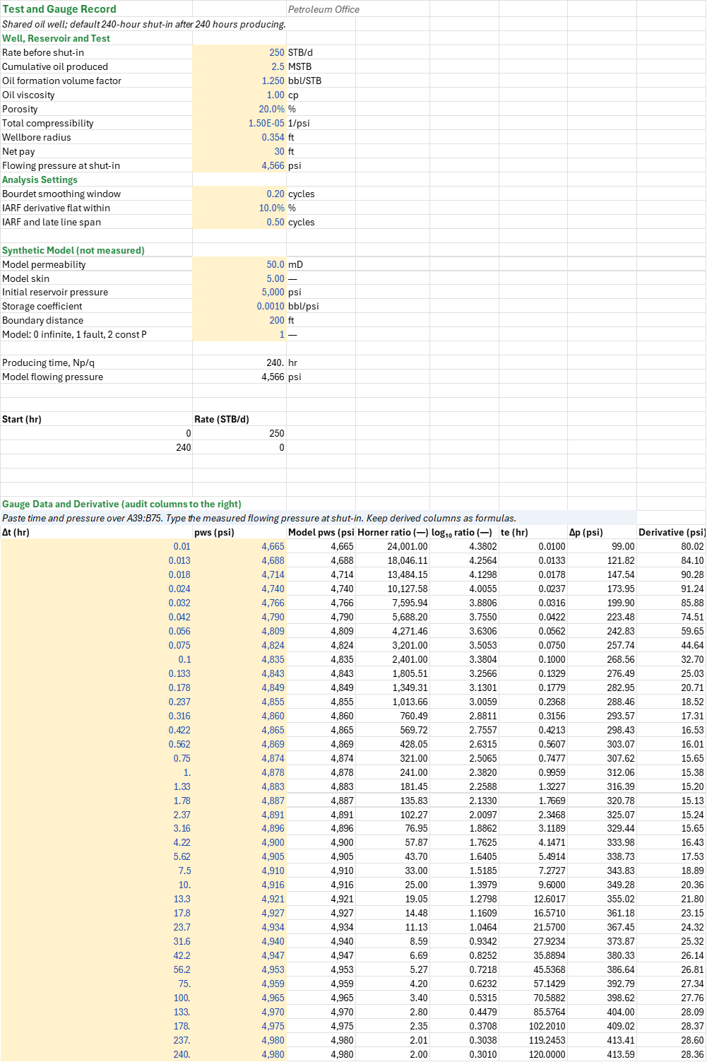
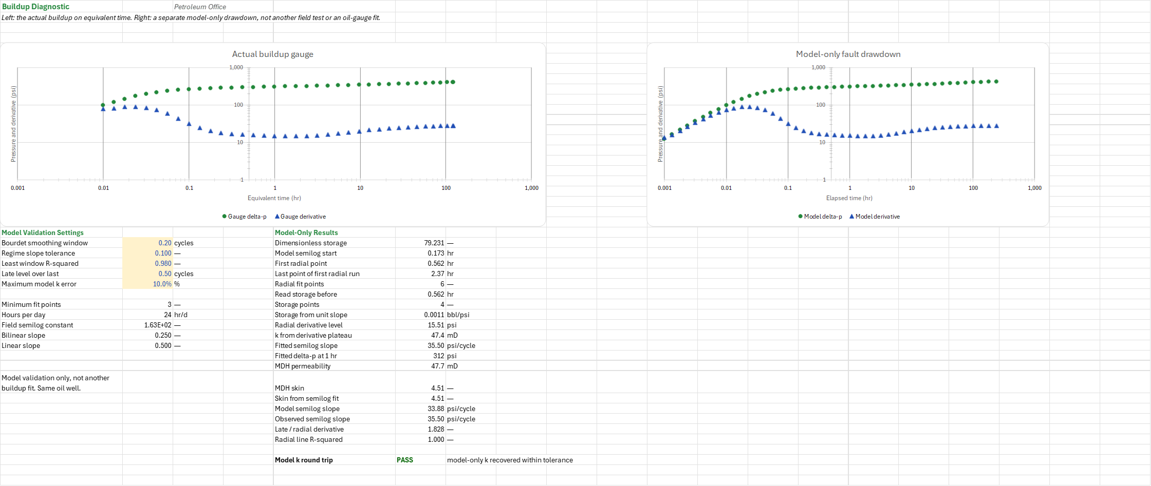
How to use it: Set q, Np and the rock and fluid properties on the Test sheet. Paste 37 positive, increasing times and pressures into A39:B75 and type the measured flowing pressure at shut-in over its model default. Leave the derived columns as formulas; changing the row count requires resizing every dependent range. Check the gauge calibration, rate stability and the derivative on the Diagnostic sheet before accepting the IARF window, then read k, skin and p-star on the Horner sheet and the late signature on the Boundary sheet. The model k, skin, pi, C and distance generate reference curves only: disregard the model round-trip checks for field data and estimate C from the early unit-slope data. The Summary is last and lists every check.
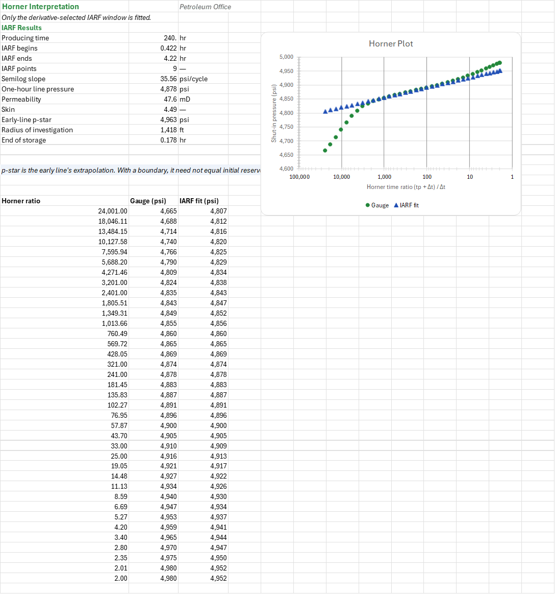
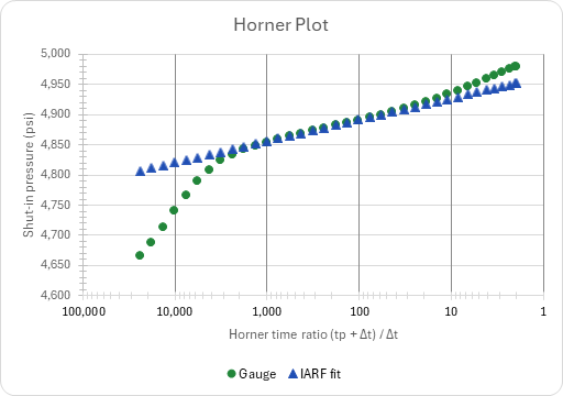
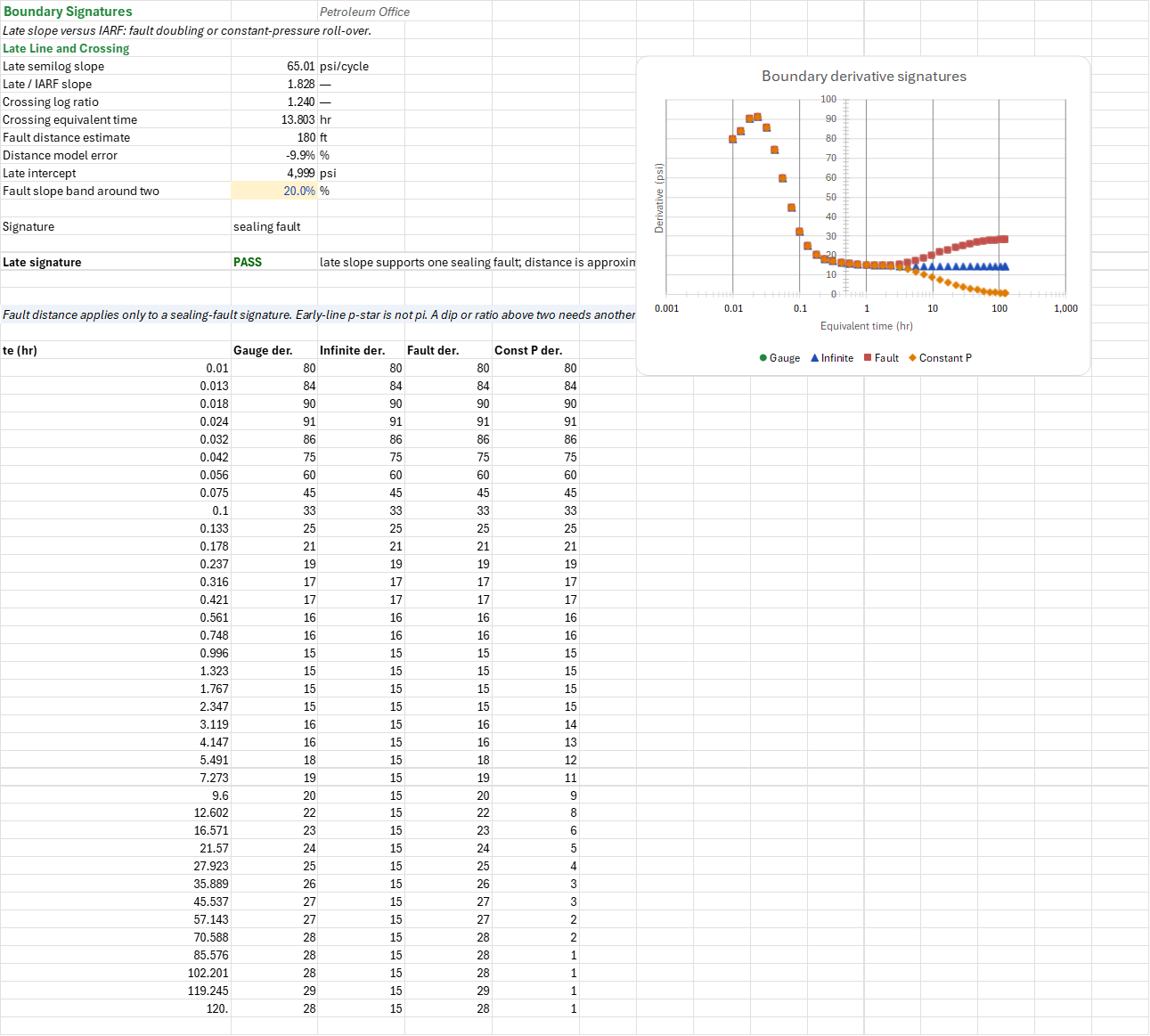
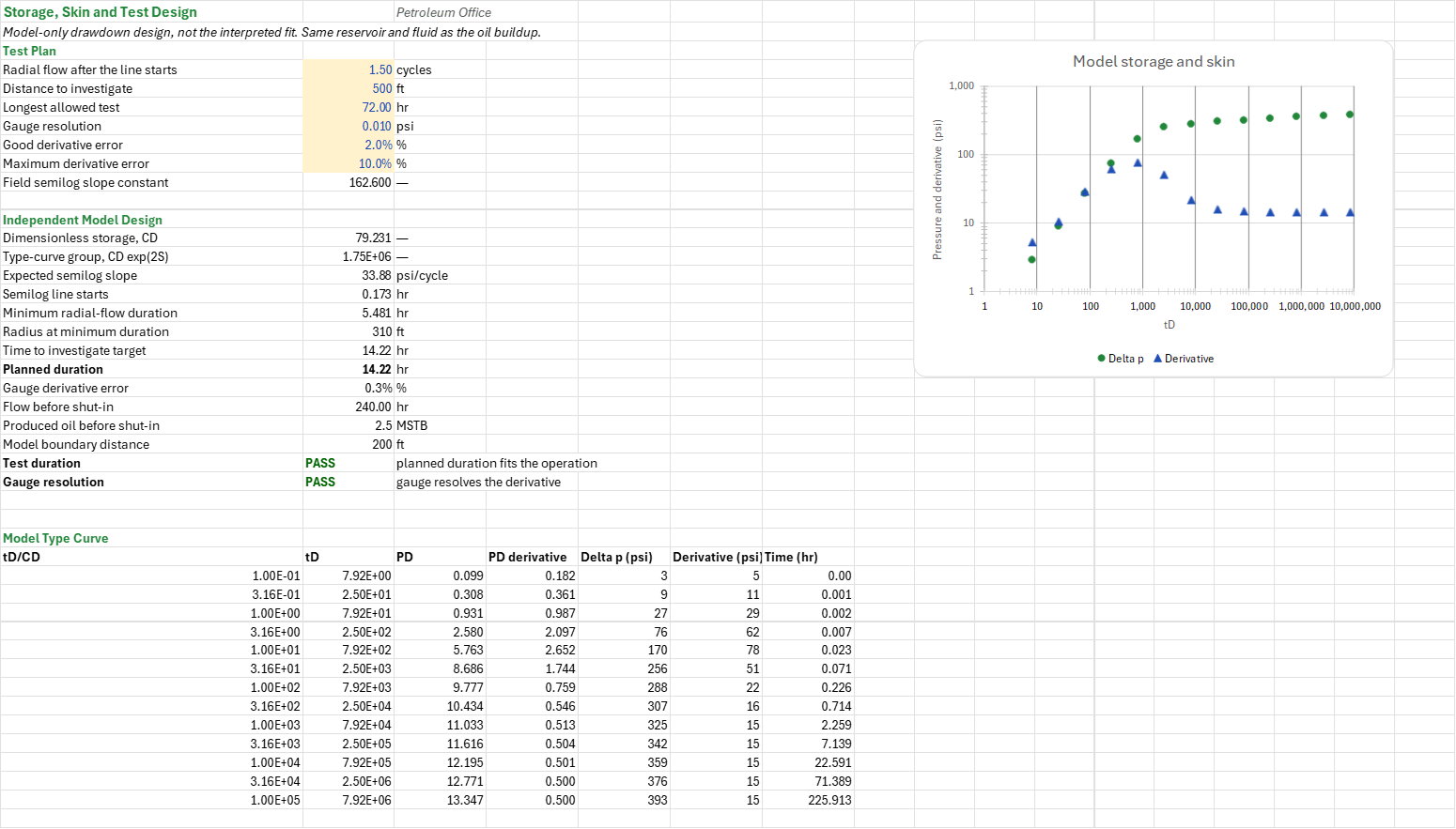
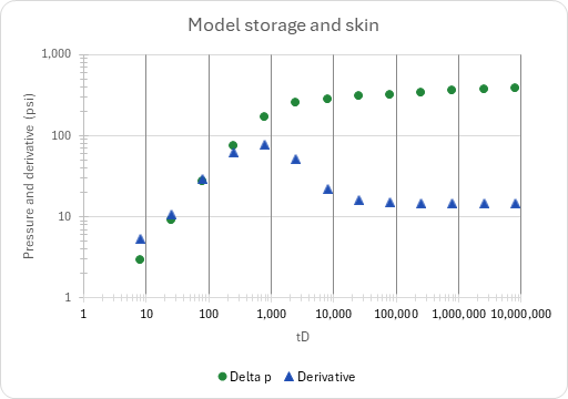
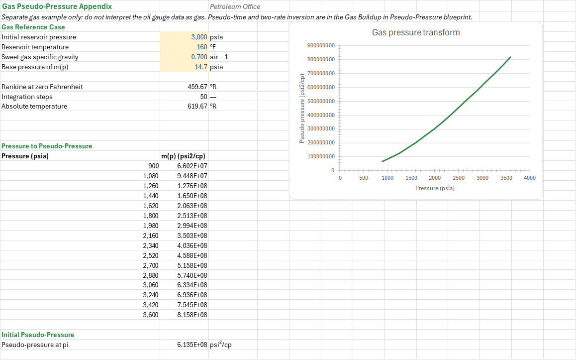
Method: Producing time is 24,000 Np/q for Np in MSTB; the Horner ratio is (tp+dt)/dt and the Agarwal equivalent time te = tp/ratio. The Bourdet derivative is d(pws-pwf)/d ln(te); multiply by LN(10) for a per-decade slope. After the storage hump, select the first connected flat run spanning at least 0.5 log10 cycle within a 10% band, and fit pws against log10(ratio) only there. Permeability is 162.6 q Bo mu/(m h); skin uses the line's one-hour pressure and the flowing pressure at shut-in; p-star is the line at ratio one. Fit the last half log cycle separately: a late/early slope ratio within 20% of two supports one sealing fault; below 0.9 supports a constant-pressure roll-over. The two lines' crossing time and the interpreted k give the fault distance. The model validation fits a Miller-Dyes-Hutchinson (MDH) line to a model drawdown and checks storage and test design. The Gas sheet integrates 2p/(mu Z) for the pseudo-pressure.
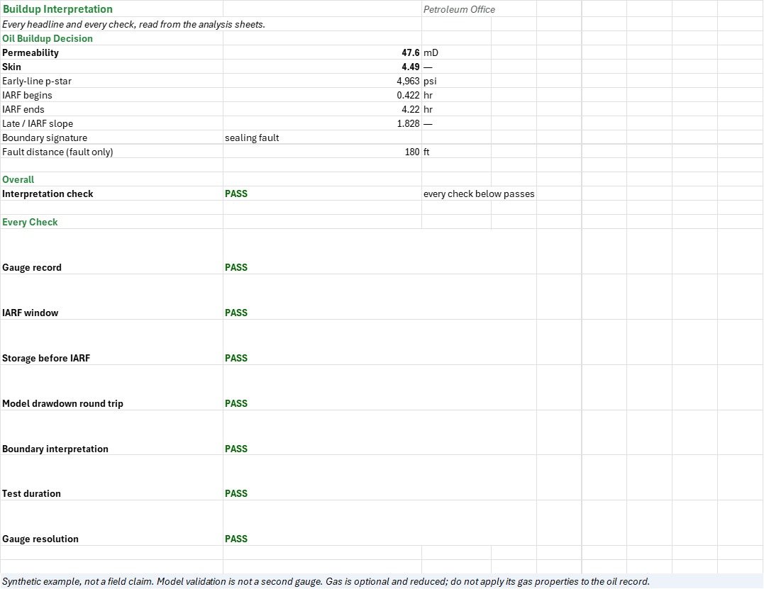
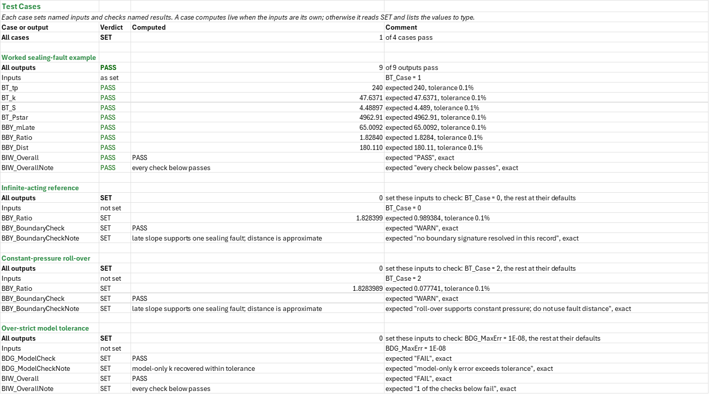
Example: The PTA reference oil well: q = 250 STB/d, Bo = 1.25 bbl/STB, mu = 1 cP, phi = 0.2, ct = 1.5e-5/psi, rw = 0.354 ft, h = 30 ft, model k = 50 mD, skin = 5, pi = 5,000 psi, C = 0.001 bbl/psi, with Np = 2.5 MSTB (tp = 240 h), a fault 200 ft away and 37 gauge points. The IARF window runs from 0.422 to 4.217 h, m = 35.5552 psi/cycle, k = 47.6371 mD, skin = 4.489 and p-star = 4,962.91 psi; the late line has m = 65.0092, a slope ratio of 1.8284, and puts the fault 180.11 ft away. These are synthetic, not field measurements. Every result matches the source calculations on identical inputs to 1e-9, including Horner on this grid. The Gas sheet keeps its source's 3,000 psia, 160 F, SG = 0.7 sweet-gas reference.
Validity
Homogeneous radial, single-phase flow with constant fluid properties, storage and skin, and one pre-shut-in rate or its Np/q equivalent. Variable rates need superposition (the DST and multi-rate workbook). Fractures, multiphase flow, dual porosity and multiple boundaries can mimic these signatures. Inspect the window: a storage tail can bias it. A finite test approaches slope doubling slowly; the default fault estimate is about 10% short. The early line's p-star need not equal the initial pressure. Use the distance only for a supported sealing-fault signature; an unresolved boundary is not proof of infinite-acting flow. Model and type curves are not another field gauge. The Gas sheet is only a 16-point m(p) lookup for a separate gas fluid, not a gas k or skin interpretation and never an interpretation of the oil gauge.
Named alternatives: nonlinear whole-record fitting and dual-porosity matching, for which the add-in has no functions. A full two-rate gas buildup, pseudo-time and inverse m(p) are left out here for size.
References
- Horner, D.R. (1951). Pressure Build-up in Wells. Proc. Third World Petroleum Congress, The Hague, Sec. II, 503-523.
- Miller, C.C., Dyes, A.B. and Hutchinson, C.A. (1950). The Estimation of Permeability and Reservoir Pressure from Bottom Hole Pressure Build-up Characteristics. Trans. AIME 189, 91-104.
- Gray, K.E. (1965). Approximating Well-to-Fault Distance from Pressure Build-up Tests. JPT 17(7), 761-767.
- Earlougher, R.C. (1977). Advances in Well Test Analysis. SPE Monograph 5.
- Agarwal, R.G. (1980). A New Method to Account for Producing Time Effects When Drawdown Type Curves Are Used to Analyze Pressure Buildup and Other Test Data. SPE-9289-MS.
- Al-Hussainy, R., Ramey, H.J. and Crawford, P.B. (1966). The Flow of Real Gases Through Porous Media. JPT 18(5), 624-636.
- Bourdet, D., Ayoub, J.A. and Pirard, Y.M. (1989). Use of Pressure Derivative in Well-Test Interpretation. SPE Formation Evaluation 4(2), 293-302. SPE-12777-PA.
Inputs
| Input | Unit | Default | Name |
|---|---|---|---|
| Rate before shut-in | STB/d | 250 | BT_q |
| Cumulative oil produced | MSTB | 2.5 | BT_Np |
| Oil formation volume factor | bbl/STB | 1.25 | BT_Bo |
| Oil viscosity | cP | 1 | BT_mu |
| Porosity | fraction | 0.2 | BT_phi |
| Total compressibility | 1/psi | 0.000015 | BT_ct |
| Wellbore radius | ft | 0.354 | BT_rw |
| Net pay | ft | 30 | BT_h |
| Flowing pressure at shut-in | psi | model | BT_Pwf |
| Shut-in times and pressures (gauge) | h, psi | model, 37 points | BT_dt, BT_Build |
| Bourdet smoothing window | natural-log cycles | 0.2 | BT_L |
| IARF derivative flat within | fraction | 0.1 | BT_Flat |
| IARF and late line span | log10 cycles | 0.5 | BT_Span |
| Model permeability | mD | 50 | BT_ModelK |
| Model skin | — | 5 | BT_ModelS |
| Initial reservoir pressure | psi | 5000 | BT_Pi |
| Storage coefficient | bbl/psi | 0.001 | BT_C |
| Boundary distance | ft | 200 | BT_Lb |
| Model: 0 infinite, 1 fault, 2 const P | choice | 1 | BT_Case |
| Fault slope band around two | fraction | 0.2 | BBY_RTol |
Sheets
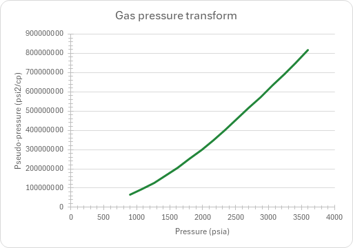
Guide— how to use the workbook, model against field data, and the reduced gas appendix and alternatives.Test— the shared test, rock, fluid and synthetic model inputs, the producing time and model flowing pressure, and the pasted gauge record with its derivative audit columns.Diagnostic— the actual buildup and its Bourdet derivative on equivalent time, the IARF window, and a separate model-only drawdown with an MDH validation fit.Horner— the Horner line through the derivative-selected IARF window only, with permeability, skin and p-star.Boundary— the late slope against the IARF slope: fault doubling or constant-pressure roll-over, and the approximate fault distance.Storage— the model-only storage and skin type curve and the test design: duration, radius of investigation and gauge resolution.Gas— a separate sweet-gas reference and its 16-point pseudo-pressure table and m(p) curve.Summary— every headline and every check.Test Cases— the worked example and other cases, with expected and computed results.
Functions used
Names (172)
| Name | Refers to | Comment |
|---|---|---|
PO.PTA.Design.DurationLAMBDA |
=LAMBDA(C, mu, k, h, S, cycles, IF((200000+12000*S)*C*mu/(k*h)<=0, NA(), (200000+12000*S)*C*mu/(k*h)*10^cycles)) |
Test duration: the start of the semilog straight line, (200000 + 12000·S)·C·μ/(k·h), carried cycles log cycles further; cycles = 0 gives the start of the line itself, [h]. |
PO.PTA.Design.GaugeResLAMBDA |
=LAMBDA(m, resolution, L, IF(OR(m<=0, L<=0), NA(), LN(10)*resolution/(L*m))) |
Gauge-resolution check: the worst-case error that a gauge resolution puts into a Bourdet derivative over a smoothing window L, as a fraction of the radial-flow derivative m/ln(10): ln(10)·resolution/(L·m), [fraction]. |
PO.PTA.Design.RinvLAMBDA |
=LAMBDA(k, t, phi, mu, ct, SQRT(k*t/(948*phi*mu*ct))) |
Radius of investigation of radial flow after t hours: sqrt(k·t / (948·φ·μ·ct)), [ft]. |
PO.PTA.MDH.FitLAMBDA |
=LAMBDA(t, dp, q, B, mu, h, phi, ct, rw, output, LET(x, LOG10(t), m, SLOPE(dp, x), dp_1h, INTERCEPT(dp, x), perm, 162.6*q*B*mu/(m*h), skin, 1.151*(dp_1h/m-LOG10(perm/(phi*mu*ct*rw^2))+3.23), IF(m<=0, NA(), IF(output="k", perm, IF(output="S", skin, IF(output="m", m, IF(output="dp1h", dp_1h, NA()))))))) |
MDH semilog straight-line fit of a drawdown: least squares of Δp against log10(t) over the points given; output "k" [mD], "S" [dimensionless], "m" [psi/cycle] or "dp1h" [psi], the line's Δp at 1 h. |
PO.PVT.PseudoPLAMBDA |
=LAMBDA(p, t_r, sg_g, p_base, steps, IF((p<p_base)+(t_r<=0)+(sg_g<=0)+(steps<1)+(p_base/PO.PVT.Ppc.BySutton(sg_g)<0.01), NA(), LET(ppc, PO.PVT.Ppc.BySutton(sg_g), tpr, t_r/PO.PVT.Tpc.BySutton(sg_g), n, INT(steps), dp, (p-p_base)/n, f, MAP(p_base+dp*SEQUENCE(n+1, 1, 0), LAMBDA(x, LET(z, PO.PVT.Z.ByDAK(x/ppc, tpr), x/(PO.PVT.Ug.ByLGE(z, sg_g, x, t_r)*z)))), 2*dp*(SUM(f)-(INDEX(f, 1)+INDEX(f, n+1))/2)))) |
Real-gas pseudo-pressure m(p) = 2*integral of p/(ug*Z) dp from p_base to p (psi2/cp), trapezoid rule in steps; Z by DAK and ug by LGE at Sutton pseudo-criticals. p, p_base psia (p_base >= 7), t_r degR, sg_g air = 1. |
_PO.PTA.EndWBSLAMBDA |
=LAMBDA(C,mu,k,h,S, (200000+12000*S)*C*mu/(k*h)) |
End of wellbore storage time, h |
_PO.PTA.FaultDistanceLAMBDA |
=LAMBDA(k,t,phi,mu,ct, SQRT(0.000148*k*t/(phi*mu*ct))) |
|
BBY_BoundaryCheck |
Boundary!$B$15 |
Late signature verdict |
BBY_BoundaryCheckNote |
Boundary!$C$15 |
Late signature comment |
BBY_CrossTe |
Boundary!$B$7 |
Crossing equivalent time, hr |
BBY_CrossX |
Boundary!$B$6 |
Crossing log ratio |
BBY_Curve |
Boundary!$A$21:$E$57 |
Boundary derivative signatures |
BBY_Dist |
Boundary!$B$8 |
Fault distance estimate, ft |
BBY_DistErr |
Boundary!$B$9 |
Distance model error, % |
BBY_IntLate |
Boundary!$B$10 |
Late intercept, psi |
BBY_RTol |
Boundary!$B$11 |
Fault slope band around two, % |
BBY_Ratio |
Boundary!$B$5 |
Late / IARF slope |
BBY_Results |
Boundary!$B$4:$B$15 |
Boundary results and verdict |
BBY_Signature |
Boundary!$B$13 |
Signature |
BBY_mLate |
Boundary!$B$4 |
Late semilog slope, psi/cycle |
BDG_Before |
Diagnostic!$F$29 |
Read storage before, hr |
BDG_CD |
Diagnostic!$F$24 |
Dimensionless storage |
BDG_CEst |
Diagnostic!$F$31 |
Storage from unit slope, bbl/psi |
BDG_FitN |
Diagnostic!$F$28 |
Radial fit points |
BDG_FitR2 |
Diagnostic!$F$42 |
Radial line R-squared |
BDG_Hr |
Diagnostic!$B$31 |
Hours per day, hr/d |
BDG_Inputs |
Diagnostic!$B$24:$B$28 |
Model-only diagnostic settings; well properties are linked to Test |
BDG_Kd |
Diagnostic!$F$33 |
k from derivative plateau, mD |
BDG_Kmdh |
Diagnostic!$F$36 |
MDH permeability, mD |
BDG_L |
Diagnostic!$B$24 |
Bourdet smoothing window, cycles |
BDG_Level |
Diagnostic!$F$32 |
Radial derivative level, psi |
BDG_MObserved |
Diagnostic!$F$40 |
Observed semilog slope, psi/cycle |
BDG_MPred |
Diagnostic!$F$39 |
Model semilog slope, psi/cycle |
BDG_MaxErr |
Diagnostic!$B$28 |
Maximum model k error, % |
BDG_Mfit |
Diagnostic!$F$34 |
Fitted semilog slope, psi/cycle |
BDG_MinN |
Diagnostic!$B$30 |
Minimum fit points |
BDG_ModelCheck |
Diagnostic!$F$44 |
Model k round trip verdict |
BDG_ModelCheckNote |
Diagnostic!$G$44 |
Model k round trip comment |
BDG_NSto |
Diagnostic!$F$30 |
Storage points |
BDG_P1fit |
Diagnostic!$F$35 |
Fitted delta-p at 1 hr, psi |
BDG_R2 |
Diagnostic!$B$26 |
Least window R-squared |
BDG_RadEnd |
Diagnostic!$F$27 |
Last point of first radial run, hr |
BDG_RadStart |
Diagnostic!$F$26 |
First radial point, hr |
BDG_Ratio |
Diagnostic!$F$41 |
Late / radial derivative |
BDG_Results |
Diagnostic!$F$24:$F$44 |
Independent model diagnostic headlines and round-trip check |
BDG_SBil |
Diagnostic!$B$33 |
Bilinear slope |
BDG_SLin |
Diagnostic!$B$34 |
Linear slope |
BDG_Sd |
Diagnostic!$F$38 |
Skin from semilog fit |
BDG_SlopeConst |
Diagnostic!$B$32 |
Field semilog constant |
BDG_Smdh |
Diagnostic!$F$37 |
MDH skin |
BDG_Span |
Diagnostic!$B$27 |
Late level over last, cycles |
BDG_TStart |
Diagnostic!$F$25 |
Model semilog start, hr |
BDG_Tol |
Diagnostic!$B$25 |
Regime slope tolerance |
BGP_Curve |
Gas!$A$17:$B$32 |
Gas pressure transform |
BGP_Inputs |
Gas!$B$4:$B$7 |
The gas blueprint's reference gas, independent of the oil gauges |
BGP_MTab |
Gas!$B$17:$B$32 |
Gas table pseudo-pressures |
BGP_MpTable |
Gas!$A$17:$B$32 |
The gas blueprint's 16 pressures from 0.3 pi to 1.2 pi and their m(p) |
BGP_PTab |
Gas!$A$17:$A$32 |
Gas table pressures |
BGP_Pbase |
Gas!$B$7 |
Base pressure of m(p), psia |
BGP_Pi |
Gas!$B$4 |
Initial reservoir pressure, psia |
BGP_R0 |
Gas!$B$9 |
Rankine at zero Fahrenheit, °R |
BGP_Results |
Gas!$B$35 |
m(pi) only; not a gas buildup interpretation |
BGP_SG |
Gas!$B$6 |
Sweet gas specific gravity, air = 1 |
BGP_Steps |
Gas!$B$10 |
Integration steps |
BGP_T |
Gas!$B$5 |
Reservoir temperature, °F |
BGP_TR |
Gas!$B$11 |
Absolute temperature, °R |
BGP_mPi |
Gas!$B$35 |
Pseudo-pressure at pi, psi²/cp |
BHN_Curve |
Horner!$A$21:$C$57 |
Horner Plot |
BHN_EndWBS |
Horner!$B$14 |
End of storage, hr |
BHN_P1hr |
Horner!$B$9 |
One-hour line pressure, psi |
BHN_Pstar |
Horner!$B$12 |
Early-line p-star, psi |
BHN_Results |
Horner!$B$4:$B$14 |
Horner results from the shared gauge and IARF fit |
BHN_Rinv |
Horner!$B$13 |
Radius of investigation, ft |
BHN_S |
Horner!$B$11 |
Skin |
BHN_WinEnd |
Horner!$B$6 |
IARF ends, hr |
BHN_WinN |
Horner!$B$7 |
IARF points |
BHN_WinStart |
Horner!$B$5 |
IARF begins, hr |
BHN_k |
Horner!$B$10 |
Permeability, mD |
BHN_m |
Horner!$B$8 |
Semilog slope, psi/cycle |
BHN_tp |
Horner!$B$4 |
Producing time, hr |
BIW_Checks |
Summary!$B$17:$B$23 |
Every check from the analysis sheets |
BIW_Distance |
Summary!$B$11 |
Fault distance (fault only), ft |
BIW_End |
Summary!$B$8 |
IARF ends, hr |
BIW_Overall |
Summary!$B$14 |
Interpretation check verdict |
BIW_OverallNote |
Summary!$C$14 |
Interpretation check comment |
BIW_Pstar |
Summary!$B$6 |
Early-line p-star, psi |
BIW_Ratio |
Summary!$B$9 |
Late / IARF slope |
BIW_Results |
Summary!$B$4:$B$14 |
Headlines and overall verdict |
BIW_S |
Summary!$B$5 |
Skin |
BIW_Signature |
Summary!$B$10 |
Boundary signature |
BIW_Start |
Summary!$B$7 |
IARF begins, hr |
BIW_k |
Summary!$B$4 |
Permeability, mD |
BST_CD |
Storage!$B$13 |
Dimensionless storage, CD |
BST_CDe2S |
Storage!$B$14 |
Type-curve group, CD exp(2S) |
BST_Curve |
Storage!$B$31:$F$43 |
Model storage and skin |
BST_Cycles |
Storage!$B$4 |
Radial flow after the line starts, cycles |
BST_DerivErr |
Storage!$B$21 |
Gauge derivative error, % |
BST_DurationCheck |
Storage!$B$25 |
Test duration verdict |
BST_DurationCheckNote |
Storage!$C$25 |
Test duration comment |
BST_GaugeCheck |
Storage!$B$26 |
Gauge resolution verdict |
BST_GaugeCheckNote |
Storage!$C$26 |
Gauge resolution comment |
BST_GoodErr |
Storage!$B$8 |
Good derivative error, % |
BST_Inputs |
Storage!$B$4:$B$9 |
Duration, radius and gauge settings of the storage blueprint |
BST_Lb |
Storage!$B$24 |
Model boundary distance, ft |
BST_M |
Storage!$B$15 |
Expected semilog slope, psi/cycle |
BST_MaxErr |
Storage!$B$9 |
Maximum derivative error, % |
BST_MaxHours |
Storage!$B$6 |
Longest allowed test, hr |
BST_Np |
Storage!$B$23 |
Produced oil before shut-in, MSTB |
BST_RTarget |
Storage!$B$5 |
Distance to investigate, ft |
BST_Resolution |
Storage!$B$7 |
Gauge resolution, psi |
BST_Results |
Storage!$B$13:$B$26 |
Model design, the shared production history and named checks |
BST_RinvMin |
Storage!$B$18 |
Radius at minimum duration, ft |
BST_SlopeConst |
Storage!$B$10 |
Field semilog slope constant |
BST_TMin |
Storage!$B$17 |
Minimum radial-flow duration, hr |
BST_TPlan |
Storage!$B$20 |
Planned duration, hr |
BST_TStart |
Storage!$B$16 |
Semilog line starts, hr |
BST_TTarget |
Storage!$B$19 |
Time to investigate target, hr |
BST_Tp |
Storage!$B$22 |
Flow before shut-in, hr |
BT_Analysis |
Test!$C$39:$N$75 |
Per row: the model pws, the Horner ratio, te, Δp, the Bourdet derivative, and the IARF window search |
BT_Bo |
Test!$B$6 |
Oil formation volume factor, bbl/STB |
BT_Build |
Test!$B$39:$B$75 |
Shut-in pressures |
BT_C |
Test!$B$22 |
Storage coefficient, bbl/psi |
BT_Case |
Test!$B$24 |
Model: 0 infinite, 1 fault, 2 const P |
BT_CoreT |
Test!$W$7 |
Flattest half cycle starts at Δt, hr |
BT_Data |
Test!$A$39:$B$75 |
The shut-in data: Δt since shut-in and the shut-in pressure (the synthetic model's until you paste a gauge's) |
BT_DataCheck |
Test!$W$31 |
Gauge record verdict |
BT_DataCheckNote |
Test!$X$31 |
Gauge record comment |
BT_EndWBS |
Test!$W$24 |
End of storage, hr |
BT_Flat |
Test!$B$15 |
IARF derivative flat within, % |
BT_From |
Test!$W$5 |
IARF search starts after Δt, hr |
BT_Inputs |
Test!$B$4:$B$24 |
Shared test, rock, fluid and synthetic model |
BT_Int |
Test!$W$28 |
IARF intercept, psi |
BT_L |
Test!$B$14 |
Bourdet smoothing window, cycles |
BT_Lb |
Test!$B$23 |
Boundary distance, ft |
BT_Level |
Test!$W$8 |
Derivative level over it, psi |
BT_ModelK |
Test!$B$19 |
Model permeability, mD |
BT_ModelS |
Test!$B$20 |
Model skin |
BT_Np |
Test!$B$5 |
Cumulative oil produced, MSTB |
BT_P1hr |
Test!$W$17 |
Line pressure at Δt = 1 hr, p1hr, psi |
BT_PErr |
Test!$W$27 |
p-star model error, psi |
BT_Peak |
Test!$W$4 |
Derivative peak (the storage hump) at Δt, hr |
BT_Pi |
Test!$B$21 |
Initial reservoir pressure, psi |
BT_Pstar |
Test!$W$20 |
Extrapolated pressure, p*, psi |
BT_Pwf |
Test!$B$12 |
Flowing pressure at shut-in, psi |
BT_PwfModel |
Test!$B$27 |
Model flowing pressure, psi |
BT_Qual |
Test!$W$6 |
Half cycles flat within the tolerance |
BT_R1hr |
Test!$W$15 |
Horner ratio at Δt = 1 hr |
BT_Rates |
Test!$A$31:$B$32 |
Rate history for the synthetic/reference model |
BT_Rinv |
Test!$W$22 |
Radius of investigation, ft |
BT_Rwa |
Test!$W$23 |
Effective wellbore radius, ft |
BT_S |
Test!$W$19 |
Skin factor, S |
BT_SErr |
Test!$W$26 |
Skin model error |
BT_Span |
Test!$B$16 |
IARF and late line span, cycles |
BT_StorageCheck |
Test!$W$30 |
Storage before IARF verdict |
BT_StorageCheckNote |
Test!$X$30 |
Storage before IARF comment |
BT_WinEnd |
Test!$W$10 |
IARF window ends at Δt, hr |
BT_WinN |
Test!$W$12 |
Points in the window |
BT_WinSpan |
Test!$W$11 |
IARF window span, cycles |
BT_WinStart |
Test!$W$9 |
IARF window starts at Δt, hr |
BT_WindowCheck |
Test!$W$29 |
IARF window verdict |
BT_WindowCheckNote |
Test!$X$29 |
IARF window comment |
BT_ct |
Test!$B$9 |
Total compressibility, 1/psi |
BT_dt |
Test!$A$39:$A$75 |
Shut-in times |
BT_h |
Test!$B$11 |
Net pay, ft |
BT_k |
Test!$W$18 |
Permeability, k, mD |
BT_kErr |
Test!$W$25 |
Permeability model error, % |
BT_m |
Test!$W$16 |
Semilog slope over the window, m, psi/cycle |
BT_mu |
Test!$B$7 |
Oil viscosity, cp |
BT_phi |
Test!$B$8 |
Porosity, % |
BT_q |
Test!$B$4 |
Rate before shut-in, STB/d |
BT_rw |
Test!$B$10 |
Wellbore radius, ft |
BT_tp |
Test!$B$26 |
Producing time, Np/q, hr |
Details
| Opens in | Needs the Petroleum Office add-in: its PO functions show #NAME? without it once Excel recalculates. Needs Microsoft 365 or Excel 2024: it uses functions Excel 2016 doesn't have, such as named LAMBDAs, which show #NAME? there. |
| File | BuildupInterpretation.xlsx, 110 KB |
| Category | Reservoir |
| For agents and tools | Descriptor (.md) |