Fracture Treatment Design
Description
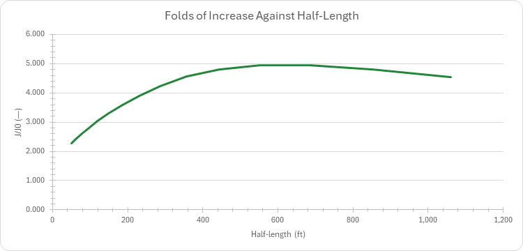
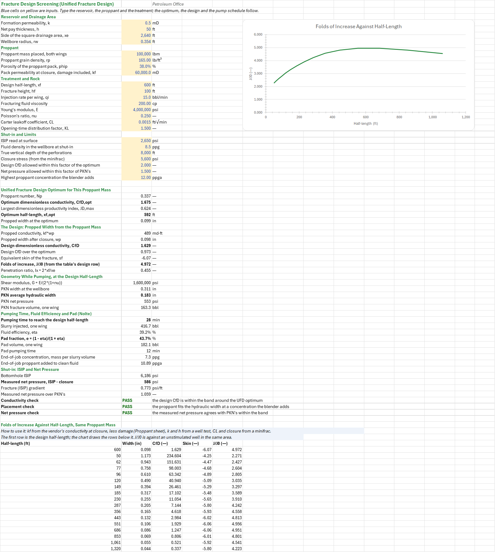
What fracture does this proppant mass buy, how do you pump it, and how much does it raise the well's productivity? You enter the reservoir and drainage area, the proppant, the rock, the fluid and leakoff, and the minifrac's closure and ISIP. You read off the optimum half-length and dimensionless conductivity, the geometry model the barriers allow, an eight-stage pump schedule, whether the proppant is carried and what conductivity survives closure, and the folds of increase. Field units; the PO add-in is needed.
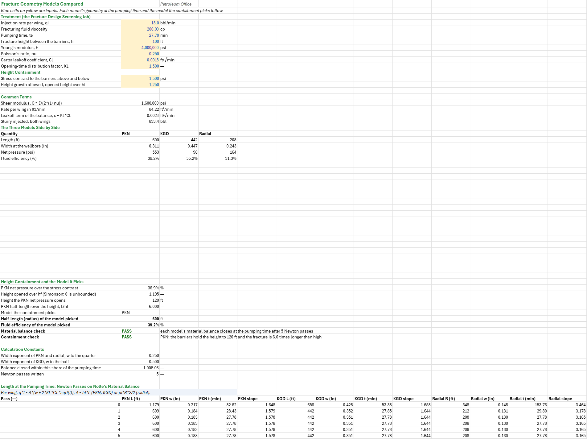
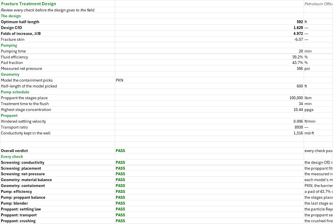
How to use it: The job is made up. On the Screening sheet, take k and h from a well test, the drainage area from the spacing, the proppant's density, pack porosity and conductivity at closure from the vendor's data, E and nu from the logs, and the leakoff coefficient and the closure from a minifrac (the DFIT workbook). Check on the Geometry sheet which model the height containment picks, then set the blender's limit from the crew on the Pump Schedule sheet and the proppant tests on the Proppant sheet. The Summary holds every headline number and the checks under one verdict.
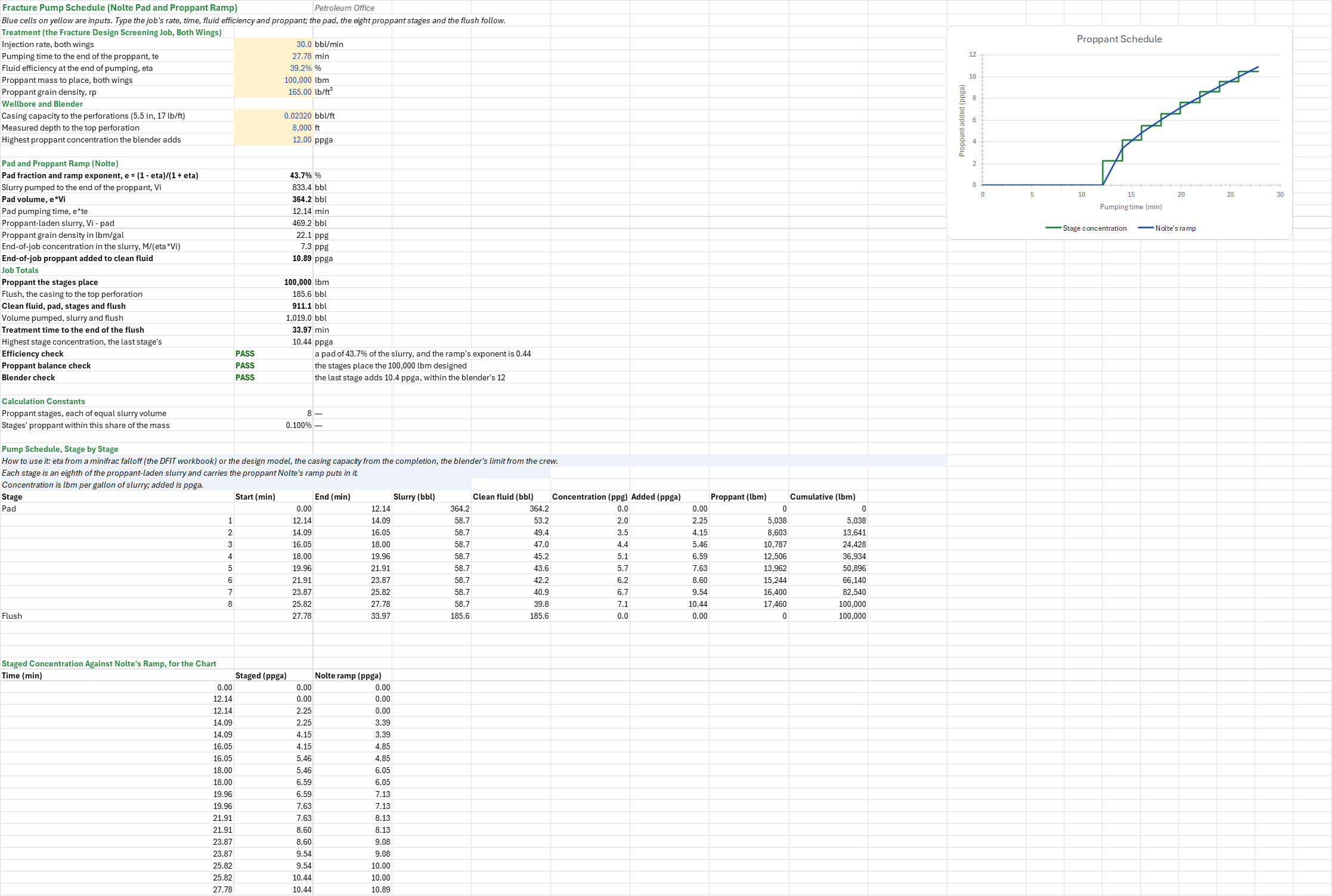
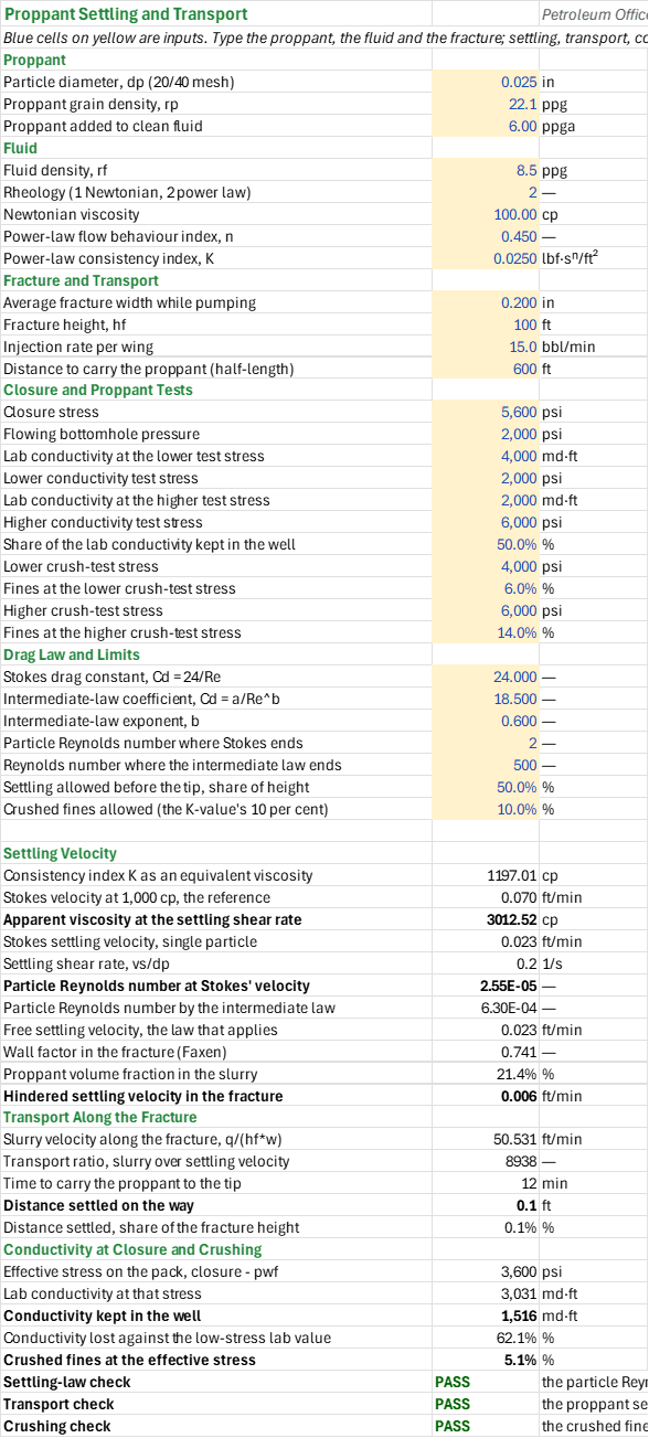
Method: The proppant number is 2 kf Vprop/(k Vres); the optimum dimensionless conductivity and half-length follow from it. The propped conductivity is kf wp, wp from the proppant mass over the propped volume, and the skin follows from wp. The folds of increase at the design half-length are (ln(xe/sqrt(pi)/rw) - 0.75) over that plus the skin. The geometry models are Nolte's material balance per wing, q t = A (w + 2 KL CL sqrt(t)), with A = hf L for PKN and KGD and pi R^2/2 for the radial fracture; each pass moves ln L by ln(te/t) over d ln t/d ln L and the balance closes in five Newton passes. The height the PKN net pressure opens between symmetric barriers (Simonson) picks the model: PKN when L/hf is at least 1, KGD when it is shorter, radial when the barriers do not hold the height. The pad fraction is (1 - eta)/(1 + eta). The proppant ramp c(x) = ce x^e gives each of the eight equal-slurry stages its share, so the stages place the designed mass exactly, and the flush follows. Settling is Stokes' in a Newtonian or a power-law fluid, replaced by the intermediate (Allen) law above the Stokes limit; the transport ratio is the slurry velocity over the settling velocity. The conductivity kept in the well at closure and the fines follow from the lab conductivity and crush tests.
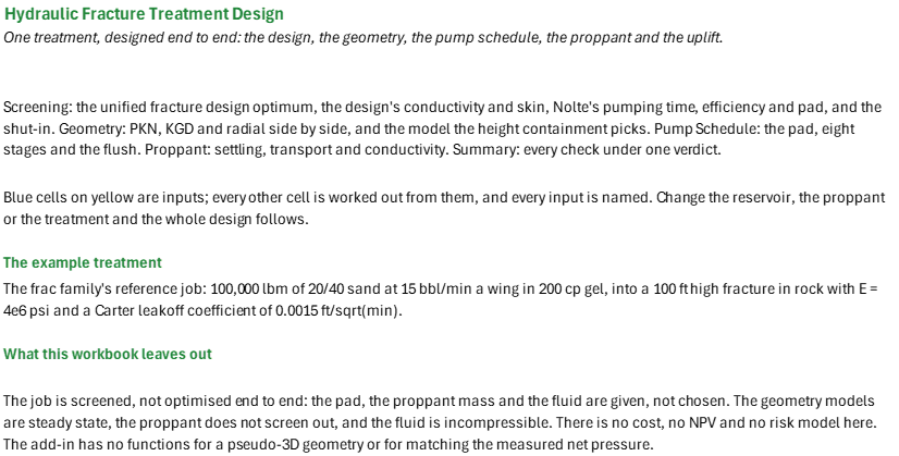
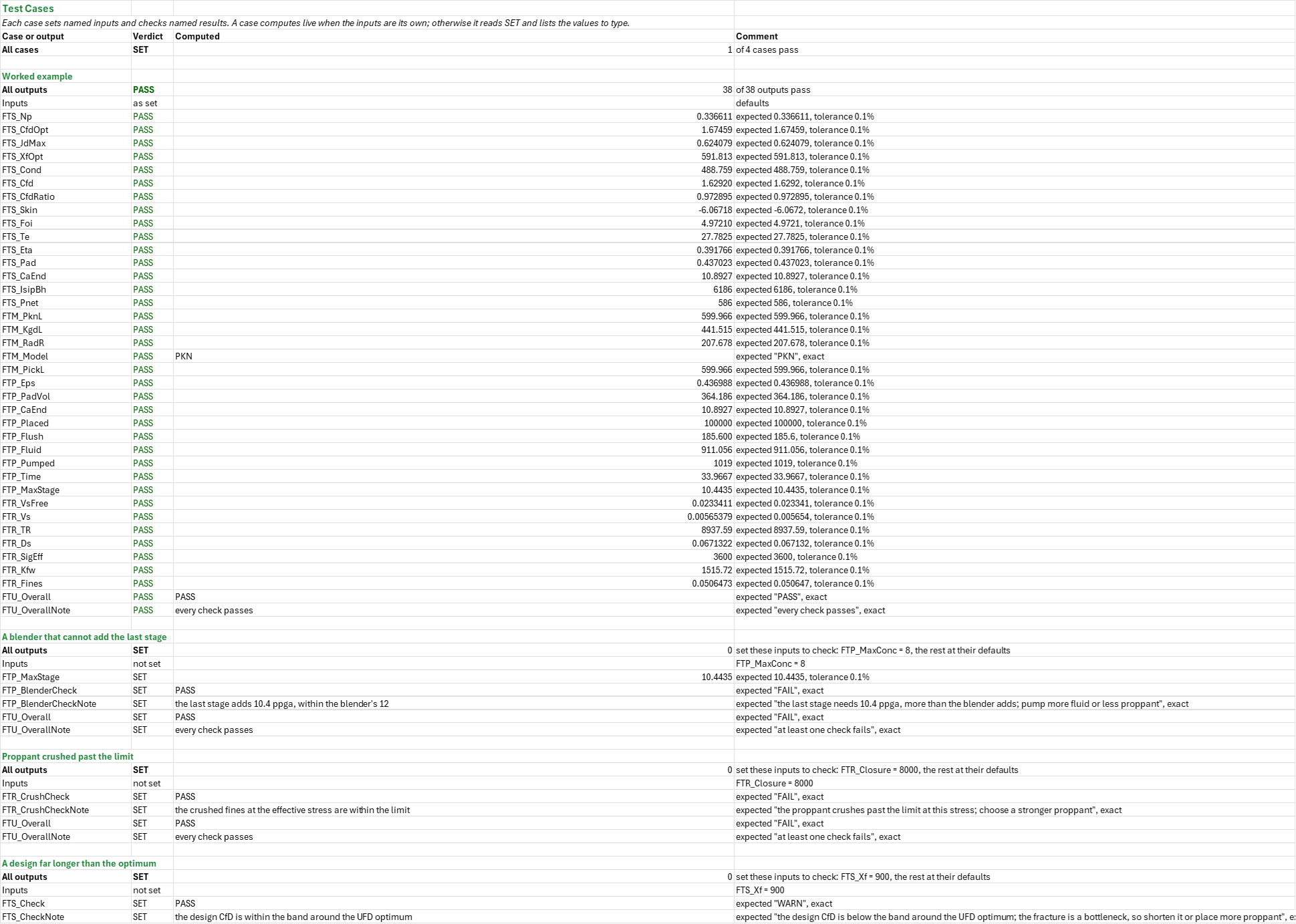
Example: The frac family's reference job, made up: 100,000 lbm of 20/40 sand at 165 lb/ft3 into a 100 ft high fracture in rock with E = 4e6 psi, pumped at 15 bbl/min a wing in 200 cp gel, with a Carter leakoff coefficient of 0.0015 ft/sqrt(min), at 8,000 ft TVD, shut in at 2,650 psi at surface with 8.5 ppg in the hole. The worked example on the Test Cases sheet checks every headline number it reaches.
Validity
The design is a screening: the proppant mass, the pad and the fluid are given, not chosen. The geometry models are steady state: the fracture does not screen out, the fluid is incompressible and non-tempered, and the leakoff is Carter's coefficient with an opening-time distribution factor. The add-in has no functions for a pseudo-3D geometry or for matching the measured net pressure against the model. The uplift is the folds of increase at the design half-length against an unstimulated well in the same area, not an economic result: there is no cost, no NPV and no risk model here. The settling assumes a rigid spherical particle. Vertical well, field units.
References
- Economides, M.J., Oligney, T.E. and Valko, P. (2002). Modern Fracture Design: Theory, Methodology, and Applications. Wiley (unified fracture design, proppant number, dimensionless conductivity).
- Economides, M.J., Watters, T.R. and Vinkelnburg, R.W. (1993). Theory of Fracture Design. Schlumberger (PKN, KGD and radial geometry).
- Nolte, R.G. and Economides, M.J. (1991). Fracturing Systems. In Reservoir Stimulation (ed. Economides and Martin), ch. 8 and 9 (material balance, proppant ramp).
- Economides, M.J. and Martin, G.P. (2007). Fracture Design and Analysis. In Reservoir Stimulation, 3rd ed. (Simonson containment).
Inputs
| Input | Unit | Default | Name |
|---|---|---|---|
| Formation permeability, k | mD | 0.5 | FTS_K |
| Net pay thickness, h | ft | 50 | FTS_H |
| Side of the square drainage area, xe | ft | 2640 | FTS_Xe |
| Wellbore radius, rw | ft | 0.354 | FTS_Rw |
| Proppant mass placed, both wings | lbm | 100000 | FTS_Mass |
| Proppant grain density, rp | lb/ft3 | 165 | FTS_RhoP |
| Porosity of the proppant pack, phip | — | 0.38 | FTS_PhiP |
| Pack permeability at closure, damage included, kf | mD | 60000 | FTS_Kf |
| Design half-length, xf | ft | 600 | FTS_Xf |
| Fracture height, hf | ft | 100 | FTS_Hf |
| Injection rate per wing, qi | bbl/min | 15 | FTS_Q |
| Fracturing fluid viscosity | cP | 200 | FTS_Mu |
| Young's modulus, E | psi | 4000000 | FTS_E |
| Poisson's ratio, nu | — | 0.25 | FTS_Nu |
| Carter leakoff coefficient, CL | ft/√min | 0.0015 | FTS_CL |
| Opening-time distribution factor, KL | — | 1.5 | FTS_KL |
| ISIP read at surface | psi | 2650 | FTS_IsipSurf |
| Fluid density in the wellbore at shut-in | ppg | 8.5 | FTS_RhoFluid |
| True vertical depth of the perforations | ft | 8000 | FTS_Tvd |
| Closure stress (from the minifrac) | psi | 5600 | FTS_Closure |
| Design CfD allowed within this factor of the optimum | — | 2 | FTS_Band |
| Net pressure allowed within this factor of PKN's | — | 1.5 | FTS_PnetBand |
| Highest proppant concentration the blender adds | ppga | 12 | FTS_MaxConc |
| Injection rate per wing, qi (Geometry) | bbl/min | 15 | FTM_Q |
| Fracturing fluid viscosity (Geometry) | cP | 200 | FTM_Mu |
| Pumping time, te | min | 27.78 | FTM_Te |
| Fracture height between the barriers, hf | ft | 100 | FTM_Hf |
| Young's modulus, E (Geometry) | psi | 4000000 | FTM_E |
| Poisson's ratio, nu (Geometry) | — | 0.25 | FTM_Nu |
| Carter leakoff coefficient, CL (Geometry) | ft/√min | 0.0015 | FTM_CL |
| Opening-time distribution factor, KL (Geometry) | — | 1.5 | FTM_KL |
| Stress contrast to the barriers above and below | psi | 1500 | FTM_Dsig |
| Height growth allowed, opened height over hf | — | 1.25 | FTM_HMax |
| Injection rate, both wings | bbl/min | 30 | FTP_Q |
| Pumping time to the end of the proppant, te | min | 27.78 | FTP_Te |
| Fluid efficiency at the end of pumping, eta | % | 0.3918 | FTP_Eta |
| Proppant mass to place, both wings | lbm | 100000 | FTP_Mass |
| Proppant grain density, rp (Pump Schedule) | lb/ft3 | 165 | FTP_RhoP |
| Casing capacity to the perforations (5.5 in, 17 lb/ft) | bbl/ft | 0.0232 | FTP_Cap |
| Measured depth to the top perforation | ft | 8000 | FTP_Md |
| Highest proppant concentration the blender adds (Pump Schedule) | ppga | 12 | FTP_MaxConc |
| Particle diameter, dp (20/40 mesh) | in | 0.025 | FTR_Dp |
| Proppant grain density, rp (Proppant) | lbm/gal | 22.07 | FTR_RhoP |
| Proppant added to clean fluid | ppga | 6 | FTR_Ca |
| Fluid density, rf | ppg | 8.5 | FTR_RhoF |
| Rheology (1 Newtonian, 2 power law) | — | 2 | FTR_Fluid |
| Newtonian viscosity | cP | 100 | FTR_Mu |
| Power-law flow behaviour index, n | — | 0.45 | FTR_N |
| Power-law consistency index, K | lbf.s/ft2 | 0.025 | FTR_Kp |
| Average fracture width while pumping | in | 0.2 | FTR_W |
| Fracture height, hf (Proppant) | ft | 100 | FTR_Hf |
| Injection rate per wing (Proppant) | bbl/min | 15 | FTR_Q |
| Distance to carry the proppant (half-length) | ft | 600 | FTR_L |
| Closure stress | psi | 5600 | FTR_Closure |
| Flowing bottomhole pressure | psi | 2000 | FTR_Pwf |
| Lab conductivity at the lower test stress | mD-ft | 4000 | FTR_KfwLo |
| Lower conductivity test stress | psi | 2000 | FTR_SigLo |
| Lab conductivity at the higher test stress | mD-ft | 2000 | FTR_KfwHi |
| Higher conductivity test stress | psi | 6000 | FTR_SigHi |
| Share of the lab conductivity kept in the well | % | 0.5 | FTR_Retained |
| Lower crush-test stress | psi | 4000 | FTR_CrushLo |
| Fines at the lower crush-test stress | % | 0.06 | FTR_FinesLo |
| Higher crush-test stress | psi | 6000 | FTR_CrushHi |
| Fines at the higher crush-test stress | % | 0.14 | FTR_FinesHi |
| Stokes drag constant, Cd = 24/Re | — | 24 | FTR_CdStokes |
| Intermediate-law coefficient, Cd = a/Re^b | — | 18.5 | FTR_CdA |
| Intermediate-law exponent, b | — | 0.6 | FTR_CdB |
| Particle Reynolds number where Stokes ends | — | 2 | FTR_ReStokes |
| Reynolds number where the intermediate law ends | — | 500 | FTR_ReMax |
| Settling allowed before the tip, share of height | % | 0.5 | FTR_SettleMax |
| Crushed fines allowed (the K-value's 10 per cent) | % | 0.1 | FTR_FinesMax |
Sheets
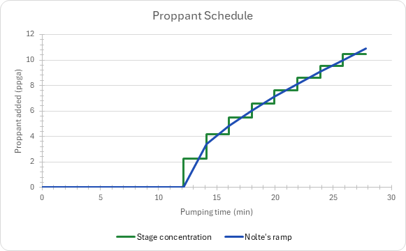
Guide— what the workbook answers, the example treatment, what it leaves out and the order to work through its sheets.Screening— unified fracture design: the proppant mass fixes the proppant number, and the optimum dimensionless conductivity and half-length follow; the design's propped width, conductivity, skin and folds of increase; the geometry while pumping, Nolte's pumping time, fluid efficiency and pad; the ISIP and net pressure at shut-in; and the folds of increase against half-length for the same proppant mass.Geometry— PKN, KGD and radial solved side by side on Nolte's material balance by Newton passes, and the Simonson height containment that picks the model.Pump Schedule— Nolte's pad and proppant ramp cut into eight equal slurry stages plus the flush, the job totals, the proppant balance and the blender limit, with the staged concentration charted against the ramp.Proppant— the proppant's settling velocity, its transport along the fracture, the conductivity kept in the well at closure and the fines the crush test gives.Summary— every headline number and the checks under one verdict.Test Cases— the worked example and other cases, with expected and computed results.
Two charts: the folds of increase on Screening, the staged concentration on Pump Schedule.
Functions used
Names (157)
| Name | Refers to | Comment |
|---|---|---|
PO.FRAC.Design.ConductivityLAMBDA |
=LAMBDA(mass, rho_p, phi_p, xf, hf, kf, IF(OR(mass<0, rho_p<=0, phi_p<0, phi_p>=1, xf<=0, hf<=0, kf<0), NA(), kf*mass/((1-phi_p)*rho_p)/(2*xf*hf))) |
Propped fracture conductivity kf·wp [md·ft] from the proppant mass: wp = mass/((1 − φp)·ρp)/(2·xf·hf), the pack spread over both wings after closure. |
PO.FRAC.Design.PadFractionLAMBDA |
=LAMBDA(eta, IF(OR(eta<=0, eta>1), NA(), (1-eta)/(1+eta))) |
Nolte's pad fraction of the slurry volume, ε = (1 − η)/(1 + η), from the fluid efficiency η; also the exponent of the proppant ramp. #N/A outside 0 < η ≤ 1. |
PO.FRAC.Design.UFDLAMBDA |
=LAMBDA(mass, rho_p, phi_p, kf, k, h, hf, xe, output, IF(OR(mass<=0, rho_p<=0, phi_p<0, phi_p>=1, kf<=0, k<=0, h<=0, hf<=0, xe<=0), NA(), LET(vbulk, mass/((1-phi_p)*rho_p), vpay, vbulk*MIN(1, h/hf), np, 2*kf*vpay/(k*xe^2*h), lnp, LN(np), cfd, IF(np<=0.1, 1.6, IF(np<=10, 1.6+EXP((-0.583+1.48*lnp)/(1+0.142*lnp)), np)), jd, IF(np<=0.1, 1/(0.99-0.5*lnp), 6/PI()-EXP((0.423-0.311*np-0.089*np^2)/(1+0.667*np+0.015*np^2))), xf, SQRT(kf*vpay/2/(cfd*h*k)), IF(output="Np", np, IF(output="CfD", cfd, IF(output="JD", jd, IF(output="xf", xf, IF(output="w", 12*vpay/2/(xf*h), NA())))))))) |
Unified fracture design: from the proppant mass, output "Np" (proppant number), "CfD" (optimum conductivity), "JD" (max productivity index), "xf" (optimum half-length, ft) or "w" (propped width, in). |
PO.FRAC.Eval.ISIPLAMBDA |
=LAMBDA(isip_surf, rho_fluid, tvd, closure, output, IF(OR(rho_fluid<0, tvd<=0), NA(), LET(isip_bh, isip_surf+0.052*rho_fluid*tvd, IF(output="ISIP", isip_bh, IF(output="Pnet", isip_bh-closure, IF(output="Gradient", isip_bh/tvd, NA())))))) |
Instantaneous shut-in pressure at the fracture from the surface ISIP plus the static column 0.052·ρ·TVD; output "ISIP" (psi), "Pnet" (ISIP − closure, psi) or "Gradient" (psi/ft). |
PO.FRAC.Proppant.ConductivityLAMBDA |
=LAMBDA(kfw_lo, sigma_lo, kfw_hi, sigma_hi, sigma_eff, retained, IF(OR(kfw_lo<=0, kfw_hi<=0, sigma_hi=sigma_lo, retained<0, retained>1), NA(), retained*kfw_lo*EXP(LN(kfw_hi/kfw_lo)*(sigma_eff-sigma_lo)/(sigma_hi-sigma_lo)))) |
Proppant pack conductivity at an effective closure stress [md·ft]: log-linear in stress through two lab points, times the share retained after gel damage, embedment and fines. |
PO.FRAC.Proppant.CrushingLAMBDA |
=LAMBDA(sigma_c, pwf, sigma_lo, fines_lo, sigma_hi, fines_hi, IF(OR(fines_lo<=0, fines_hi<=0, sigma_hi=sigma_lo), NA(), MIN(1, fines_lo*EXP(LN(fines_hi/fines_lo)*(MAX(0, sigma_c-pwf)-sigma_lo)/(sigma_hi-sigma_lo))))) |
Crushed fines (fraction) at the pack's effective stress, closure less flowing pressure: log-linear in stress through two crush-test points (ISO 13503-2), capped at 1. |
FTM_CL |
Geometry!$B$10 |
|
FTM_Compare |
Geometry!$A$23:$D$26 |
|
FTM_Dsig |
Geometry!$B$13 |
|
FTM_E |
Geometry!$B$8 |
|
FTM_HMax |
Geometry!$B$14 |
|
FTM_Hf |
Geometry!$B$7 |
|
FTM_Inputs |
Geometry!$B$4:$B$14 |
|
FTM_KL |
Geometry!$B$11 |
|
FTM_KgdL |
Geometry!$C$23 |
|
FTM_Model |
Geometry!$B$51 |
|
FTM_ModelCheck |
Geometry!$B$55 |
|
FTM_ModelCheckNote |
Geometry!$C$55 |
|
FTM_Mu |
Geometry!$B$5 |
|
FTM_Nu |
Geometry!$B$9 |
|
FTM_Passes |
Geometry!$B$61 |
|
FTM_PickEta |
Geometry!$B$53 |
|
FTM_PickL |
Geometry!$B$52 |
|
FTM_PknL |
Geometry!$B$23 |
|
FTM_Q |
Geometry!$B$4 |
|
FTM_RadR |
Geometry!$D$23 |
|
FTM_Results |
Geometry!$B$17:$B$55 |
|
FTM_SolveCheck |
Geometry!$B$54 |
|
FTM_SolveCheckNote |
Geometry!$C$54 |
|
FTM_SolveTol |
Geometry!$B$60 |
|
FTM_Solver |
Geometry!$A$66:$M$71 |
|
FTM_Te |
Geometry!$B$6 |
|
FTP_BalTol |
'Pump Schedule'!$B$36 |
|
FTP_BalanceCheck |
'Pump Schedule'!$B$31 |
|
FTP_BalanceCheckNote |
'Pump Schedule'!$C$31 |
|
FTP_BlenderCheck |
'Pump Schedule'!$B$32 |
|
FTP_BlenderCheckNote |
'Pump Schedule'!$C$32 |
|
FTP_CaEnd |
'Pump Schedule'!$B$22 |
|
FTP_Cap |
'Pump Schedule'!$B$10 |
|
FTP_Eps |
'Pump Schedule'!$B$15 |
|
FTP_Eta |
'Pump Schedule'!$B$6 |
|
FTP_EtaCheck |
'Pump Schedule'!$B$30 |
|
FTP_EtaCheckNote |
'Pump Schedule'!$C$30 |
|
FTP_Fluid |
'Pump Schedule'!$B$26 |
|
FTP_Flush |
'Pump Schedule'!$B$25 |
|
FTP_Inputs |
'Pump Schedule'!$B$4:$B$12 |
|
FTP_Mass |
'Pump Schedule'!$B$7 |
|
FTP_MaxConc |
'Pump Schedule'!$B$12 |
|
FTP_MaxStage |
'Pump Schedule'!$B$29 |
|
FTP_Md |
'Pump Schedule'!$B$11 |
|
FTP_PadVol |
'Pump Schedule'!$B$17 |
|
FTP_Placed |
'Pump Schedule'!$B$24 |
|
FTP_Pumped |
'Pump Schedule'!$B$27 |
|
FTP_Q |
'Pump Schedule'!$B$4 |
|
FTP_Ramp |
'Pump Schedule'!$A$58:$C$75 |
|
FTP_Results |
'Pump Schedule'!$B$15:$B$32 |
|
FTP_RhoP |
'Pump Schedule'!$B$8 |
|
FTP_Stages |
'Pump Schedule'!$A$43:$I$52 |
|
FTP_Te |
'Pump Schedule'!$B$5 |
|
FTP_Time |
'Pump Schedule'!$B$28 |
|
FTR_Ca |
Proppant!$B$6 |
|
FTR_CdA |
Proppant!$B$32 |
|
FTR_CdB |
Proppant!$B$33 |
|
FTR_CdStokes |
Proppant!$B$31 |
|
FTR_Check |
Proppant!$B$63 |
|
FTR_CheckNote |
Proppant!$C$63 |
|
FTR_Closure |
Proppant!$B$19 |
|
FTR_CrushCheck |
Proppant!$B$65 |
|
FTR_CrushCheckNote |
Proppant!$C$65 |
|
FTR_CrushHi |
Proppant!$B$28 |
|
FTR_CrushLo |
Proppant!$B$26 |
|
FTR_Dp |
Proppant!$B$4 |
|
FTR_Ds |
Proppant!$B$55 |
|
FTR_Fines |
Proppant!$B$62 |
|
FTR_FinesHi |
Proppant!$B$29 |
|
FTR_FinesLo |
Proppant!$B$27 |
|
FTR_FinesMax |
Proppant!$B$37 |
|
FTR_Fluid |
Proppant!$B$9 |
|
FTR_Hf |
Proppant!$B$15 |
|
FTR_Inputs |
Proppant!$B$4:$B$37 |
|
FTR_Kfw |
Proppant!$B$60 |
|
FTR_KfwHi |
Proppant!$B$23 |
|
FTR_KfwLo |
Proppant!$B$21 |
|
FTR_Kp |
Proppant!$B$12 |
|
FTR_L |
Proppant!$B$17 |
|
FTR_Mu |
Proppant!$B$10 |
|
FTR_N |
Proppant!$B$11 |
|
FTR_Pwf |
Proppant!$B$20 |
|
FTR_Q |
Proppant!$B$16 |
|
FTR_ReMax |
Proppant!$B$35 |
|
FTR_ReStokes |
Proppant!$B$34 |
|
FTR_Results |
Proppant!$B$40:$B$65 |
|
FTR_Retained |
Proppant!$B$25 |
|
FTR_RhoF |
Proppant!$B$8 |
|
FTR_RhoP |
Proppant!$B$5 |
|
FTR_SettleMax |
Proppant!$B$36 |
|
FTR_SigEff |
Proppant!$B$58 |
|
FTR_SigHi |
Proppant!$B$24 |
|
FTR_SigLo |
Proppant!$B$22 |
|
FTR_TR |
Proppant!$B$53 |
|
FTR_TransportCheck |
Proppant!$B$64 |
|
FTR_TransportCheckNote |
Proppant!$C$64 |
|
FTR_Vs |
Proppant!$B$50 |
|
FTR_VsFree |
Proppant!$B$47 |
|
FTR_W |
Proppant!$B$14 |
|
FTS_Band |
Screening!$B$27 |
|
FTS_CL |
Screening!$B$20 |
|
FTS_CaEnd |
Screening!$B$59 |
|
FTS_Cfd |
Screening!$B$40 |
|
FTS_CfdOpt |
Screening!$B$33 |
|
FTS_CfdRatio |
Screening!$B$41 |
|
FTS_Check |
Screening!$B$65 |
|
FTS_CheckNote |
Screening!$C$65 |
|
FTS_Closure |
Screening!$B$26 |
|
FTS_Cond |
Screening!$B$38 |
|
FTS_Curve |
Screening!$A$73:$E$89 |
|
FTS_E |
Screening!$B$18 |
|
FTS_Eta |
Screening!$B$54 |
|
FTS_Foi |
Screening!$B$43 |
|
FTS_H |
Screening!$B$5 |
|
FTS_Hf |
Screening!$B$15 |
|
FTS_Inputs |
Screening!$B$4:$B$29 |
|
FTS_IsipBh |
Screening!$B$61 |
|
FTS_IsipSurf |
Screening!$B$23 |
|
FTS_JdMax |
Screening!$B$34 |
|
FTS_K |
Screening!$B$4 |
|
FTS_KL |
Screening!$B$21 |
|
FTS_Kf |
Screening!$B$12 |
|
FTS_Mass |
Screening!$B$9 |
|
FTS_MaxConc |
Screening!$B$29 |
|
FTS_Mu |
Screening!$B$17 |
|
FTS_Np |
Screening!$B$32 |
|
FTS_Nu |
Screening!$B$19 |
|
FTS_Pad |
Screening!$B$55 |
|
FTS_PhiP |
Screening!$B$11 |
|
FTS_PknPnet |
Screening!$B$49 |
|
FTS_PlaceCheck |
Screening!$B$66 |
|
FTS_PlaceCheckNote |
Screening!$C$66 |
|
FTS_Pnet |
Screening!$B$62 |
|
FTS_PnetBand |
Screening!$B$28 |
|
FTS_PnetCheck |
Screening!$B$67 |
|
FTS_PnetCheckNote |
Screening!$C$67 |
|
FTS_Q |
Screening!$B$16 |
|
FTS_Results |
Screening!$B$32:$B$67 |
|
FTS_RhoFluid |
Screening!$B$24 |
|
FTS_RhoP |
Screening!$B$10 |
|
FTS_Rw |
Screening!$B$7 |
|
FTS_Skin |
Screening!$B$42 |
|
FTS_Te |
Screening!$B$52 |
|
FTS_Tvd |
Screening!$B$25 |
|
FTS_Xe |
Screening!$B$6 |
|
FTS_Xf |
Screening!$B$14 |
|
FTS_XfOpt |
Screening!$B$35 |
|
FTU_Checks |
Summary!$B$28:$B$38 |
|
FTU_Overall |
Summary!$B$26 |
|
FTU_OverallNote |
Summary!$C$26 |
|
FTU_Results |
Summary!$B$4:$B$23 |
Details
| Opens in | Needs the Petroleum Office add-in: its PO functions show #NAME? without it once Excel recalculates. Needs Microsoft 365 or Excel 2024: it uses functions Excel 2016 doesn't have, such as named LAMBDAs, which show #NAME? there. |
| File | FracTreatmentDesign.xlsx, 60 KB |
| Category | Drilling |
| For agents and tools | Descriptor (.md) |