Shaly-Sand Water Saturation
Description
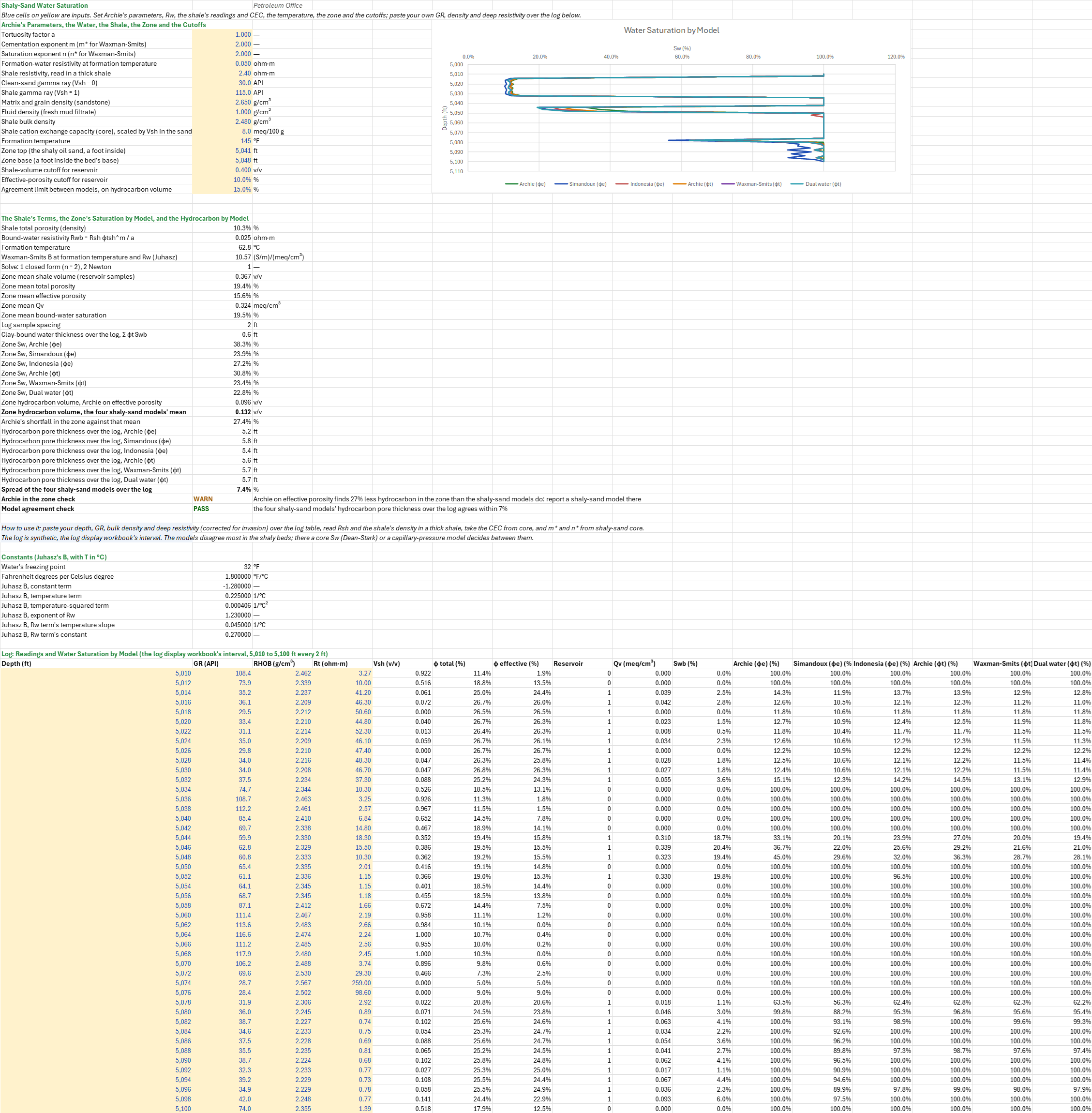
How much water is in a shaly sand, and how much does the model change the answer? In a shaly sand the clay conducts as well as the brine, so Archie reads too much water. You enter Archie's parameters, Rw, the shale's resistivity, density and cation exchange capacity, the formation temperature, a zone and the cutoffs, over a gamma-ray, density and deep-resistivity log. You read off water saturation at every depth by Simandoux, Indonesia, Waxman-Smits, dual water and Archie, and the hydrocarbon each model finds in the zone and over the log.
Parameters:
- Archie:
SS_a,SS_m,SS_n(m* and n* for Waxman-Smits) and Rw at formation temperatureSS_Rw(ohm·m) - Shale: its resistivity
SS_Rsh(ohm·m), the gamma-ray picksSS_GRcl,SS_GRsh(API), its bulk densitySS_RhoSh(g/cm³) and its cation exchange capacitySS_CECsh(meq/100 g) - Rock and temperature: the matrix and grain density
SS_RhoMaand fluid densitySS_RhoF(g/cm³), and the formation temperatureSS_Tf(°F) - Zone and cutoffs: the zone's top and base
SS_ZTop,SS_ZBase(ft), the reservoir cutoffs on shale volumeSS_VshCutand effective porositySS_PhiCut, and the agreement limitSS_Tol - Log: depth, GR, bulk density and deep resistivity in the log table, every 2 ft
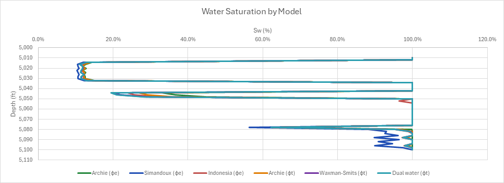
How to use it: The log is synthetic. Paste your depth, gamma ray, bulk density and deep resistivity (corrected for invasion) over the log table. Read Rsh and the shale's density in a thick shale on the same log. Take the CEC from core, scaled to the sand by its shale volume or measured on it, and m* and n* from shaly-sand core. Where the models disagree, a core saturation (Dean-Stark) or a capillary-pressure model decides between them. A log track draws Sw by all six against depth.
Method: The models fall in two families. The shale-volume models, Simandoux and Indonesia, add a conductive shale of resistivity Rsh in proportion to Vsh. They work on effective porosity and reduce to Archie on effective porosity with no shale. The clay-conductance models work on total porosity and reduce to Archie on total porosity with no clay. Waxman-Smits puts the clay's conductivity in its exchange cations, Qv from the cation exchange capacity, with B from Juhasz's fit at formation temperature. Dual water treats the clay-bound water as a second water of its own resistivity Rwb. Both Archies are on the sheet, each beside the models that reduce to it. Their saturations are of different porosities, so the comparison is on the hydrocarbon each model finds, φ (1 − Sw) in its own porosity, a volume of rock that does not depend on the porosity it is counted in.
- Shale volume and porosity. Vsh is the linear gamma-ray index, kept between 0 and 1. Total porosity is the density porosity φt = (ρma − ρb) / (ρma − ρf), and the shale's total porosity φtsh is the same from its density. Effective porosity is φe = φt − Vsh φtsh. A sample is reservoir when Vsh is at most the cutoff and φe at least its cutoff; any other sample reads Sw = 1.
- Archie: Sw = (a Rw / (φ^m Rt))^(1/n), on φe and on φt.
- Simandoux: Sw = (0.4 Rw / φe²) [−Vsh/Rsh + √((Vsh/Rsh)² + 5 φe² / (Rw Rt))].
- Indonesia: 1/√Rt = [Vsh^(1 − Vsh/2) / √Rsh + φe^(m/2) / √(a Rw)] Sw^(n/2).
- Waxman-Smits: 1/Rt = (φt^m / a) (Sw^n / Rw + B Qv Sw^(n−1)). Qv = CEC (1 − φt) ρg / (100 φt), with the sand's CEC Vsh × CECsh. B is Juhasz's fit, B = (−1.28 + 0.225 T − 0.0004059 T²) / (1 + Rw^1.23 (0.045 T − 0.27)), T in °C.
- Dual water: 1/Rt = (φt^m Sw^n / a) [1/Rw + (1/Rwb − 1/Rw) Swb/Sw]. The bound water's resistivity is Rwb = Rsh φtsh^m / a, the shale's water, and its saturation Swb = Vsh φtsh / φt.
- Solution. Waxman-Smits and dual water are solved in closed form at n = 2 and by Newton's method otherwise. Each saturation is shown at most 1. The zone's values are the means of its reservoir samples. The hydrocarbon pore thickness of a model is Σ φ (1 − Sw) times the sample spacing, in that model's porosity.
- Checks. Two checks give PASS or WARN. The Archie check warns when Archie on effective porosity finds less hydrocarbon in the zone than the shaly-sand models' mean by more than the agreement limit. The agreement check warns when the four shaly-sand models' hydrocarbon pore thickness over the log spreads by more than that limit.
Example: The default case is the Well-Log Display workbook's synthetic interval, from 5,010 to 5,100 ft every 2 ft: the reservoir part, from the shale above the clean oil sand to the shale below the water sand. Its parameters are the workbook's: a, m and n of 1, 2 and 2, Rw 0.05 ohm·m and Rsh 2.4 ohm·m, gamma-ray picks of 30 and 115 API, a 2.65 g/cm³ sandstone and 1.0 g/cm³ filtrate, and reservoir cutoffs of 0.40 Vsh and 10% effective porosity. The shale reads 2.48 g/cm³, and its CEC is taken as 8 meq/100 g, an illitic shale. The formation is at 145°F. The zone is the shaly sand above its oil–water contact, a foot inside its top and base, 5,041 to 5,048 ft. The models have to agree within 15%.
The shale's total porosity is (2.65 − 2.48) / 1.65 = 10.3%, so Rwb = 2.4 × 0.1030² = 0.0255 ohm·m. At 145°F, 62.8°C, Juhasz's B is (−1.28 + 14.125 − 1.600) / (1 + 0.0251 × 2.555) = 10.57 (S/m)/(meq/cm³). In the zone, 5,042 ft is above the 0.40 Vsh cutoff, so three samples count, from 5,044 to 5,048 ft. Their mean Vsh is 0.367, total porosity 19.4%, effective porosity 15.6%, Qv 0.324 meq/cm³ and bound-water saturation 19.5%. Archie on effective porosity reads 38.3% water. Simandoux reads 23.9% and Indonesia 27.2%. On total porosity Archie reads 30.8%, Waxman-Smits 23.4% and dual water 22.8%. In hydrocarbon volume Archie on effective porosity finds 0.096 against the four shaly-sand models' mean of 0.132, 27% less: the Archie check warns, which is the point of the sheet. Over the log the clean oil sand carries most of the hydrocarbon, where the models agree. The pore thickness is 5.24 ft by Archie on effective porosity and 5.59 ft on total porosity, 5.85 ft by Simandoux, 5.43 ft by Indonesia, 5.73 ft by Waxman-Smits and 5.75 ft by dual water. The four shaly-sand models spread 7%, within 15%, so the agreement check passes. With no CEC, Waxman-Smits reads the zone as Archie on total porosity does, 30.8%. In the clean oil sand from 5,013 to 5,033 ft Archie is within the limit and the Archie check passes. A 5% agreement limit makes the agreement check warn. At n = 2.2 Waxman-Smits and dual water are solved by Newton's method and read 27.5% and 27.0%, against 34.3% by Archie on total porosity.
Functions used
None: the blueprint calculates with Excel's own functions.
Names (68)
| Name | Refers to | Comment |
|---|---|---|
PO.PP.Vsh.GammaRayIndexLAMBDA |
=LAMBDA(GR, GR_cl, GR_sh, (GR-GR_cl)/(GR_sh-GR_cl)) |
Linear gamma-ray shale index, IGR = (GR - GRclean) / (GRshale - GRclean). |
PO.PP.Porosity.FromDensityLAMBDA |
=LAMBDA(Rho_ma, Rho_b, Rho_f, (Rho_ma-Rho_b)/(Rho_ma-Rho_f)) |
Porosity from a density log, (matrix density - bulk density) / (matrix density - fluid density). |
PO.PP.Sw.ArchieLAMBDA |
=LAMBDA(a, m, n, Phi, Rw, Rt, ((a/Phi^m)*(Rw/Rt))^(1/n)) |
Water saturation from the general Archie equation, Sw = ((a/phi^m)*(Rw/Rt))^(1/n). |
PO.PP.Sw.SimandouxLAMBDA |
=LAMBDA(Phi_e, Rt, Rw, Vsh, Rsh, (0.4*Rw/Phi_e^2)*(-Vsh/Rsh+SQRT((Vsh/Rsh)^2+5*Phi_e^2/(Rw*Rt)))) |
Simandoux (1963) water saturation for a shaly sand, Bassiouni's a = 0.8 and m = 2 form. |
PO.PP.Sw.IndonesiaLAMBDA |
=LAMBDA(a, m, n, Phi_e, Rw, Rt, Vsh, Rsh, POWER(1/(SQRT(Rt)*(Vsh^(1-Vsh/2)/SQRT(Rsh)+Phi_e^(m/2)/SQRT(a*Rw))), 2/n)) |
Indonesia (Poupon-Leveaux 1971) water saturation for a shaly formation. |
PO.PP.Qv.FromCECLAMBDA |
=LAMBDA(CEC, PhiT_frac, Rho_g, CEC*(1-PhiT_frac)*Rho_g/(100*PhiT_frac)) |
Cation exchange capacity per unit pore volume, Qv = CEC (1 - phi) rho_g / (100 phi), meq/cm3, from CEC in meq/100 g. |
PO.PP.Sw.WaxmanSmitsLAMBDA |
=LAMBDA(a, m, n, Phi, Rw, Rt, B, Qv, Mode, LET(ct, 1/Rt, cw, 1/Rw, kf, Phi^m/a, bq, B*Qv, IF(Mode=1, IF(n=2, (-bq+SQRT(bq^2+4*cw*ct/kf))/(2*cw), NA()), IF(Mode=2, REDUCE(1, SEQUENCE(30), LAMBDA(s, j, s-(kf*(cw*s^n+bq*s^(n-1))-ct)/(kf*(n*cw*s^(n-1)+(n-1)*bq*s^(n-2))))), NA())))) |
Waxman-Smits (1968) water saturation from Qv and B: Mode 1 the quadratic closed form (n = 2 only), Mode 2 a 30-step Newton solve for any n. |
PO.PP.Sw.DualWaterLAMBDA |
=LAMBDA(a, m, n, Phi_t, Rw, Rwb, Swb, Rt, Mode, LET(ct, 1/Rt, cw, 1/Rw, kf, Phi_t^m/a, bq, (1/Rwb-1/Rw)*Swb, swt, IF(Mode=1, IF(n=2, (-bq+SQRT(bq^2+4*cw*ct/kf))/(2*cw), NA()), IF(Mode=2, REDUCE(1, SEQUENCE(30), LAMBDA(s, j, s-(kf*(cw*s^n+bq*s^(n-1))-ct)/(kf*(n*cw*s^(n-1)+(n-1)*bq*s^(n-2))))), NA())), HSTACK(swt, (swt-Swb)/(1-Swb)))) |
Dual-water (Clavier et al. 1984) saturation: {Swt, Swe}. Mode 1 the quadratic closed form (n = 2 only), Mode 2 a 30-step Newton solve for any n. |
SS_a |
$B$4 |
Tortuosity factor a |
SS_m |
$B$5 |
Cementation exponent m (m* for Waxman-Smits) |
SS_n |
$B$6 |
Saturation exponent n (n* for Waxman-Smits) |
SS_Rw |
$B$7 |
Formation-water resistivity at formation temperature, ohm·m |
SS_Rsh |
$B$8 |
Shale resistivity, read in a thick shale, ohm·m |
SS_GRcl |
$B$9 |
Clean-sand gamma ray (Vsh = 0), API |
SS_GRsh |
$B$10 |
Shale gamma ray (Vsh = 1), API |
SS_RhoMa |
$B$11 |
Matrix and grain density (sandstone), g/cm³ |
SS_RhoF |
$B$12 |
Fluid density (fresh mud filtrate), g/cm³ |
SS_RhoSh |
$B$13 |
Shale bulk density, g/cm³ |
SS_CECsh |
$B$14 |
Shale cation exchange capacity (core), scaled by Vsh in the sand, meq/100 g |
SS_Tf |
$B$15 |
Formation temperature, °F |
SS_ZTop |
$B$16 |
Zone top (the shaly oil sand, a foot inside), ft |
SS_ZBase |
$B$17 |
Zone base (a foot inside the bed's base), ft |
SS_VshCut |
$B$18 |
Shale-volume cutoff for reservoir, v/v |
SS_PhiCut |
$B$19 |
Effective-porosity cutoff for reservoir, % |
SS_Tol |
$B$20 |
Agreement limit between models, on hydrocarbon volume, % |
SS_Inputs |
$B$4:$B$20 |
Archie's a, m and n, Rw, Rsh, the gamma-ray picks, the matrix, fluid and shale densities, the shale's CEC, the formation temperature, the zone, the reservoir cutoffs and the agreement limit |
SS_PhiTsh |
$B$24 |
Shale total porosity (density), % |
SS_Rwb |
$B$25 |
Bound-water resistivity Rwb = Rsh φtsh^m / a, ohm·m |
SS_TfC |
$B$26 |
Formation temperature, °C |
SS_B |
$B$27 |
Waxman-Smits B at formation temperature and Rw (Juhasz), (S/m)/(meq/cm³) |
SS_Mode |
$B$28 |
Solve: 1 closed form (n = 2), 2 Newton |
SS_ZVsh |
$B$29 |
Zone mean shale volume (reservoir samples), v/v |
SS_ZPhiT |
$B$30 |
Zone mean total porosity, % |
SS_ZPhiE |
$B$31 |
Zone mean effective porosity, % |
SS_ZQv |
$B$32 |
Zone mean Qv, meq/cm³ |
SS_ZSwb |
$B$33 |
Zone mean bound-water saturation, % |
SS_Step |
$B$34 |
Log sample spacing, ft |
SS_Bound |
$B$35 |
Clay-bound water thickness over the log, Σ φt Swb, ft |
SS_ZSwA |
$B$36 |
Zone Sw, Archie (φe), % |
SS_ZSwS |
$B$37 |
Zone Sw, Simandoux (φe), % |
SS_ZSwI |
$B$38 |
Zone Sw, Indonesia (φe), % |
SS_ZSwT |
$B$39 |
Zone Sw, Archie (φt), % |
SS_ZSwW |
$B$40 |
Zone Sw, Waxman-Smits (φt), % |
SS_ZSwD |
$B$41 |
Zone Sw, Dual water (φt), % |
SS_ZHcA |
$B$42 |
Zone hydrocarbon volume, Archie on effective porosity, v/v |
SS_ZHcShaly |
$B$43 |
Zone hydrocarbon volume, the four shaly-sand models' mean, v/v |
SS_Short |
$B$44 |
Archie's shortfall in the zone against that mean, % |
SS_HcA |
$B$45 |
Hydrocarbon pore thickness over the log, Archie (φe), ft |
SS_HcS |
$B$46 |
Hydrocarbon pore thickness over the log, Simandoux (φe), ft |
SS_HcI |
$B$47 |
Hydrocarbon pore thickness over the log, Indonesia (φe), ft |
SS_HcT |
$B$48 |
Hydrocarbon pore thickness over the log, Archie (φt), ft |
SS_HcW |
$B$49 |
Hydrocarbon pore thickness over the log, Waxman-Smits (φt), ft |
SS_HcD |
$B$50 |
Hydrocarbon pore thickness over the log, Dual water (φt), ft |
SS_Spread |
$B$51 |
Spread of the four shaly-sand models over the log, % |
SS_ArchieCheck |
$B$52 |
Archie in the zone check verdict |
SS_ArchieCheckNote |
$C$52 |
Archie in the zone check comment |
SS_SpreadCheck |
$B$53 |
Model agreement check verdict |
SS_SpreadCheckNote |
$C$53 |
Model agreement check comment |
SS_Results |
$B$24:$B$53 |
Shale porosity, Rwb, temperature, B and the solve, the zone's shale volume, porosities, Qv, bound water and Sw by each model, hydrocarbon by Archie and the shaly-sand models, clay-bound water, HC pore thickness by model, their spread, two checks |
SS_TfZero |
$B$59 |
Water's freezing point, °F |
SS_TfPerC |
$B$60 |
Fahrenheit degrees per Celsius degree, °F/°C |
SS_J1 |
$B$61 |
Juhasz B, constant term |
SS_J2 |
$B$62 |
Juhasz B, temperature term, 1/°C |
SS_J3 |
$B$63 |
Juhasz B, temperature-squared term, 1/°C² |
SS_J4 |
$B$64 |
Juhasz B, exponent of Rw |
SS_J5 |
$B$65 |
Juhasz B, Rw term's temperature slope, 1/°C |
SS_J6 |
$B$66 |
Juhasz B, Rw term's constant |
SS_Curve |
$A$70:$P$115 |
Each depth's GR, density and deep resistivity, its shale volume, total and effective porosity, reservoir flag, Qv, bound-water saturation and Sw by each of the six models |
Details
| Inserts | 115 rows × 16 columns |
| Category | Petrophysics |
| For agents and tools | Descriptor (.md) |