Type Well Curves
Description
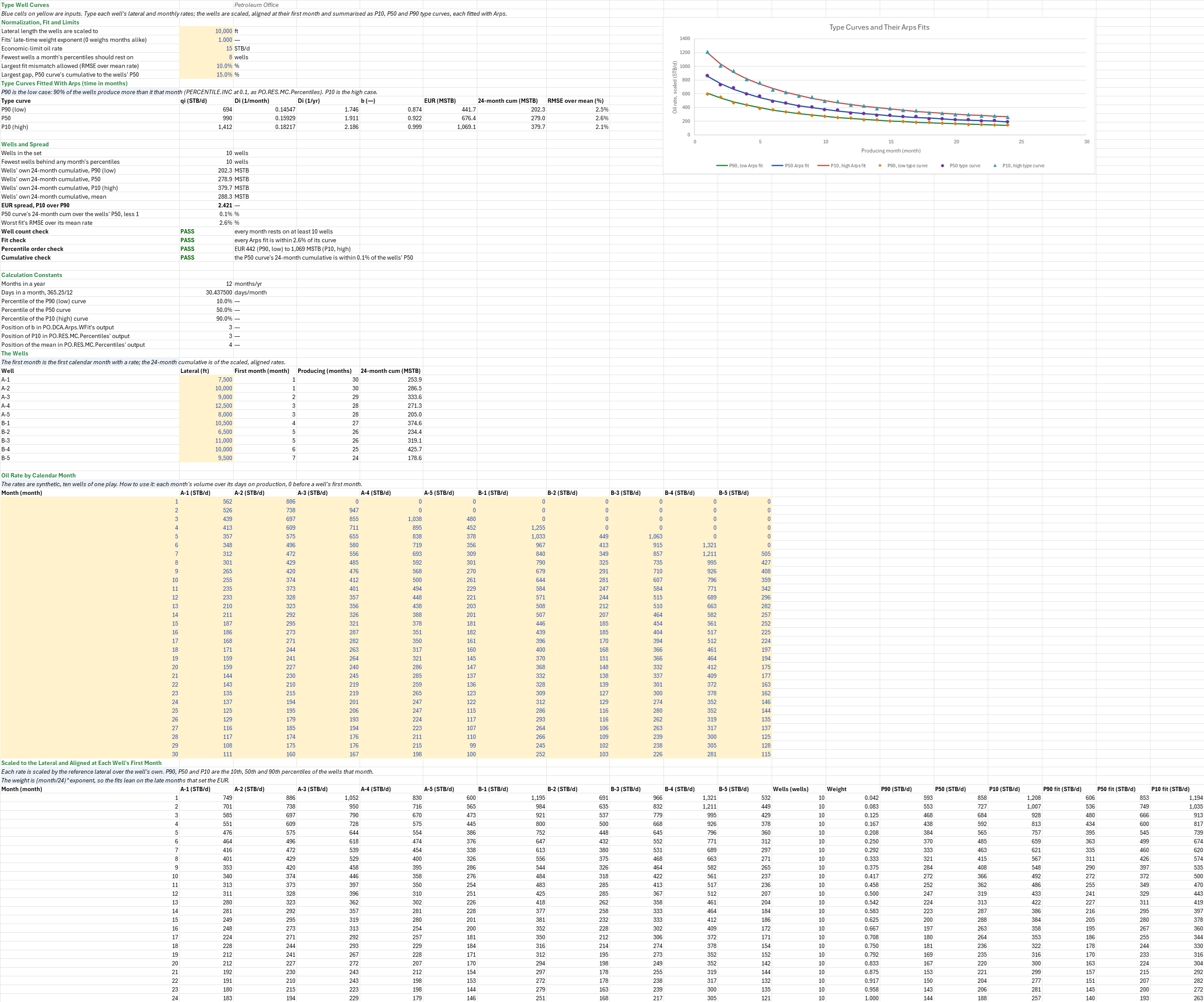
What does a new well in this play produce, low, mid and high? You enter a set of wells' monthly oil rates by calendar month and their lateral lengths, a reference lateral and an economic-limit rate. Each well is scaled to the reference lateral and aligned at its own first month. You read off the P90, P50 and P10 type curves, each curve's Arps qi, Di, b and EUR, and how the curves' 24-month cumulatives compare with the wells' own.
Parameters:
- Normalization: the lateral length the wells are scaled to,
TW_RefLat(ft) - Fits: the late-time weight exponent
TW_WPow(the weight is (month/24)^exponent; 0 weighs every month alike) and the economic-limit rateTW_QEcon(STB/d) - Limits: the fewest wells a month's percentiles should rest on
TW_MinWells, the largest fit mismatchTW_FitMax, and the largest gap between the P50 curve's 24-month cumulative and the wells' P50TW_CumBand - Wells: each well's lateral length (ft) and its oil rate (STB/d) in calendar months 1 to 30, 0 before it came online
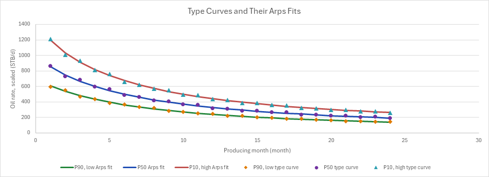
How to use it: Take each well's monthly volume over its days on production, from its first full month; leave out wells with a frac hit, a long shut-in or a recompletion in their first 24 months, or the percentiles will mix two populations. Use wells of one landing zone, completion design and vintage, and at least eight to ten of them. Scale by lateral only where the play shows rate in proportion to completed length; otherwise type a reference lateral equal to the wells' own. Check that every month rests on enough wells, that each fit matches its curve, that the three EURs come in order, and that the P50 curve's cumulative is close to the wells' P50. The chart draws the three type curves and their three fits; it leaves the individual wells off, which keeps it to six series.
Method: A well's first month (time zero) is the first calendar month with a rate. Its rate in producing month k is its rate in calendar month first + k − 1, times the reference lateral over its own. The P90, P50 and P10 rates at month k are the wells' 10th, 50th and 90th percentiles, Excel's PERCENTILE.INC of the ten scaled rates at 0.1, 0.5 and 0.9: the values sorted and read at position p·(n − 1) from the first, interpolating between neighbours. The convention is the reserves one: P90 is the low case, the rate 90 % of the wells exceed that month (at 0.1), and P10 the high case (at 0.9). Statistical software names them the other way round. Each curve is fitted with Arps, q = qi/(1 + b·Di·t)^(1/b) with t in months, by a weighted least-squares fit in log rate with the late-time weights; Di per year is twelve times Di per month. The EUR is the Arps cumulative to the economic limit, times 365.25/12 days a month. A curve's 24-month cumulative is the sum of its monthly rates times the days in a month, and a well's the same over its scaled rates; the wells' cumulatives are summarised by the same percentile convention. A curve of percentiles is not one well: the P50 curve takes each month's median, which can be a different well from month to month.
Example: The default set is synthetic: ten tight-oil horizontals of one play, with laterals of 6,500 to 12,500 ft, brought online over the first seven of 30 calendar months. Each is an Arps hyperbolic in its own months (60 to 160 STB/d of qi per 1,000 ft of lateral, Di 1.65 to 2.25/yr, b 0.85 to 1.02) with a fixed ±4 % scatter, rounded to the barrel; the median well is close to the decline family's reference well (1,020 STB/d, 1.89/yr, 0.93 at 10,000 ft). The economic limit is 15 STB/d and the late-time weight exponent 1, as on the Decline Model Auto-Fit sheet.
All ten wells have 24 months or more, so every month rests on ten. The P90 (low) curve starts at 593 STB/d and fits qi 694.5 STB/d, Di 1.746/yr, b 0.874, for an EUR of 442 MSTB; the P50 starts at 858 STB/d, fits 989.9 STB/d, 1.912/yr, 0.922, EUR 676 MSTB; the P10 (high) starts at 1,208 STB/d, fits 1,411.8 STB/d, 2.186/yr, 0.999, EUR 1,069 MSTB. The P10 EUR is 2.42 times the P90's. Every fit is within 2.6 % of its curve. The wells' own 24-month cumulatives are 202.3 (P90), 278.9 (P50) and 379.7 MSTB (P10), mean 288.3 MSTB; the P50 curve's is 279.0 MSTB, 0.06 % off. These wells keep their rank from month to month, which is why the curves' cumulatives match the wells' so closely.
Functions used
PO.DCA.Arps.WFit(times, rates, weights)
Fit Arps decline to rate-time data with weights and return parameters as a column array (Qi, Di, b).
PO.DCA.Arps.EUR(Qi, Di, b, Q_econ)
Estimated Ultimate Recovery (EUR) to an economic rate limit for Arps decline, {L3}. Returns cumulative production up to the time the rate reaches the economic limit.
PO.Stats.RMSE(observed, predicted)
Computes the root mean squared error (RMSE) between observed and predicted sequences. RMSE = sqrt(SSE/n).
PO.DCA.Arps.Rate(Qi, Di, b, time)
Calculates rate using Arps (1945) decline curve, {L3/T}. Units of volume {L3} and time {T} must be consistent. Use b=0 for exponential, 0<b<1 for hyperbolic, b=1 for harmonic.
Names (71)
| Name | Refers to | Comment |
|---|---|---|
PO.RES.MC.PercentilesLAMBDA |
=LAMBDA(X, HSTACK(PERCENTILE.INC(X, 0.1), PERCENTILE.INC(X, 0.5), PERCENTILE.INC(X, 0.9), AVERAGE(X))) |
P90, P50, P10 (petroleum convention: P90 the low case, exceeded 90% of the time) and the mean of a column of outcomes; linear interpolation as PERCENTILE.INC. |
TW_RefLat |
$B$4 |
Lateral length the wells are scaled to, ft |
TW_WPow |
$B$5 |
Fits' late-time weight exponent (0 weighs months alike) |
TW_QEcon |
$B$6 |
Economic-limit oil rate, STB/d |
TW_MinWells |
$B$7 |
Fewest wells a month's percentiles should rest on, wells |
TW_FitMax |
$B$8 |
Largest fit mismatch allowed (RMSE over mean rate), % |
TW_CumBand |
$B$9 |
Largest gap, P50 curve's cumulative to the wells' P50, % |
TW_Inputs |
$B$4:$B$9 |
The lateral the wells are scaled to, the fits' late-time weight exponent, the economic limit, the fewest wells a month needs, the fit mismatch allowed and the cumulative gap allowed |
TW_MoYr |
$B$33 |
Months in a year, months/yr |
TW_DMo |
$B$34 |
Days in a month, 365.25/12, days/month |
TW_PLow |
$B$35 |
Percentile of the P90 (low) curve |
TW_PMid |
$B$36 |
Percentile of the P50 curve |
TW_PHigh |
$B$37 |
Percentile of the P10 (high) curve |
TW_BPos |
$B$38 |
Position of b in PO.DCA.Arps.WFit's output |
TW_P10Pos |
$B$39 |
Position of P10 in PO.RES.MC.Percentiles' output |
TW_MeanPos |
$B$40 |
Position of the mean in PO.RES.MC.Percentiles' output |
TW_Wells |
$A$44:$E$53 |
Each well's name and lateral length, its first producing calendar month, its producing months and its scaled 24-month cumulative |
TW_Lat |
$B$44:$B$53 |
Each well's lateral length, ft |
TW_Cums |
$E$44:$E$53 |
Each well's scaled 24-month cumulative, MSTB |
TW_Calendar |
$A$58:$K$87 |
Each well's oil rate in each calendar month, 0 before it came online |
TW_M |
$A$58:$A$87 |
Calendar months, 1 to 30 |
TW_Aligned |
$A$92:$S$115 |
Each producing month, each well's rate scaled to the reference lateral, the wells that month, the fits' weight, the P90, P50 and P10 rates and the three Arps fits |
TW_K |
$A$92:$A$115 |
Producing months, 1 to 24 |
TW_Count |
$L$92:$L$115 |
Wells with a rate in each producing month |
TW_W |
$M$92:$M$115 |
The fits' weight for each month |
TW_P90 |
$N$92:$N$115 |
The P90 (low) type curve's rate each month, STB/d |
TW_FitP90 |
$Q$92:$Q$115 |
The P90 (low) Arps fit's rate each month, STB/d |
TW_P50 |
$O$92:$O$115 |
The P50 type curve's rate each month, STB/d |
TW_FitP50 |
$R$92:$R$115 |
The P50 Arps fit's rate each month, STB/d |
TW_P10 |
$P$92:$P$115 |
The P10 (high) type curve's rate each month, STB/d |
TW_FitP10 |
$S$92:$S$115 |
The P10 (high) Arps fit's rate each month, STB/d |
TW_Fits |
$A$13:$H$15 |
Each type curve's Arps qi, Di per month and per year and b, its EUR to the economic limit, its 24-month cumulative and its fit's RMSE over its mean rate |
TW_P90Qi |
$B$13 |
P90 type curve's fitted qi, STB/d |
TW_P90DiM |
$C$13 |
P90 type curve's fitted Di, 1/month |
TW_P90Di |
$D$13 |
P90 type curve's fitted Di, 1/yr |
TW_P90B |
$E$13 |
P90 type curve's fitted b |
TW_P90EUR |
$F$13 |
P90 type curve's EUR to the economic limit, MSTB |
TW_P90Cum |
$G$13 |
P90 type curve's 24-month cumulative, MSTB |
TW_P90Err |
$H$13 |
P90 fit's RMSE over the curve's mean rate |
TW_P50Qi |
$B$14 |
P50 type curve's fitted qi, STB/d |
TW_P50DiM |
$C$14 |
P50 type curve's fitted Di, 1/month |
TW_P50Di |
$D$14 |
P50 type curve's fitted Di, 1/yr |
TW_P50B |
$E$14 |
P50 type curve's fitted b |
TW_P50EUR |
$F$14 |
P50 type curve's EUR to the economic limit, MSTB |
TW_P50Cum |
$G$14 |
P50 type curve's 24-month cumulative, MSTB |
TW_P50Err |
$H$14 |
P50 fit's RMSE over the curve's mean rate |
TW_P10Qi |
$B$15 |
P10 type curve's fitted qi, STB/d |
TW_P10DiM |
$C$15 |
P10 type curve's fitted Di, 1/month |
TW_P10Di |
$D$15 |
P10 type curve's fitted Di, 1/yr |
TW_P10B |
$E$15 |
P10 type curve's fitted b |
TW_P10EUR |
$F$15 |
P10 type curve's EUR to the economic limit, MSTB |
TW_P10Cum |
$G$15 |
P10 type curve's 24-month cumulative, MSTB |
TW_P10Err |
$H$15 |
P10 fit's RMSE over the curve's mean rate |
TW_NWells |
$B$18 |
Wells in the set, wells |
TW_NMin |
$B$19 |
Fewest wells behind any month's percentiles, wells |
TW_CumP90 |
$B$20 |
Wells' own 24-month cumulative, P90 (low), MSTB |
TW_CumP50 |
$B$21 |
Wells' own 24-month cumulative, P50, MSTB |
TW_CumP10 |
$B$22 |
Wells' own 24-month cumulative, P10 (high), MSTB |
TW_CumMean |
$B$23 |
Wells' own 24-month cumulative, mean, MSTB |
TW_EurRatio |
$B$24 |
EUR spread, P10 over P90 |
TW_CumGap |
$B$25 |
P50 curve's 24-month cum over the wells' P50, less 1, % |
TW_WorstErr |
$B$26 |
Worst fit's RMSE over its mean rate, % |
TW_WellsCheck |
$B$27 |
Well count check verdict |
TW_WellsCheckNote |
$C$27 |
Well count check comment |
TW_FitCheck |
$B$28 |
Fit check verdict |
TW_FitCheckNote |
$C$28 |
Fit check comment |
TW_OrderCheck |
$B$29 |
Percentile order check verdict |
TW_OrderCheckNote |
$C$29 |
Percentile order check comment |
TW_CumCheck |
$B$30 |
Cumulative check verdict |
TW_CumCheckNote |
$C$30 |
Cumulative check comment |
TW_Results |
$B$18:$B$30 |
The wells in the set and the fewest behind any month, the wells' own 24-month cumulative percentiles and mean, the EUR spread, the P50 curve's gap to the wells' P50, the worst fit, and the four checks |
Details
| Inserts | 115 rows × 19 columns |
| Category | Decline Curve Analysis |
| For agents and tools | Descriptor (.md) |