CO2 Storage Capacity of a Saline Formation

Description
How much CO2 can a saline formation hold, and can wells get it in? You enter the formation's area, thickness, porosity and depth, its pressure and temperature gradients, the storage efficiency's percentiles, the rock's injectivity and the project's rate and period. You read off the CO2 density, the DOE/NETL volumetric capacity with its sampled P90, P50 and P10, the injection rate per well and the wells the project needs, and whether the capacity holds the project's CO2.
Parameters:
- Formation: the area
CS_Area(km²), the gross thicknessCS_H(m), the total porosityCS_Phiand the depth to its middleCS_Z(m) - Gradients: the pore-pressure gradient
CS_PGrad(kPa/m), the surface temperatureCS_TSurf(°C) and the geothermal gradientCS_TGrad(°C/km) - Efficiency: the storage efficiency's 10th, 50th and 90th percentiles
CS_E10,CS_E50andCS_E90 - Injectivity: the permeability
CS_K(mD), the CO2 end-point relative permeabilityCS_Kr, the net thickness open to injectionCS_HInj(m), the fracture gradientCS_FGrad(kPa/m) and the fraction of it the well may reachCS_SF, and the radiiCS_ReandCS_Rw(m) - Project: the injection rate
CS_Rate(Mt/yr) and periodCS_Years - Trials:
CS_n, a whole number from 10 to 1,000, and the permutation multiplierCS_Mult - Limits: the fewest trials
CS_NMin, the largest gap between the sampled and the DOE P90 and P10CS_Tol, and the lowest rate per wellCS_MinRate
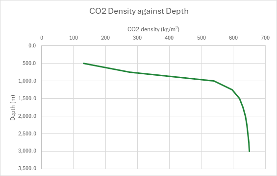
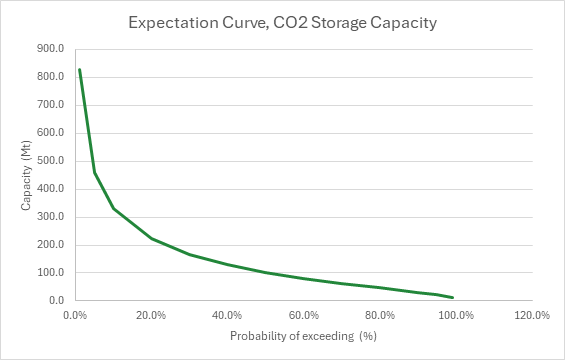
How to use it: The default aquifer is synthetic. Take the area, gross thickness and porosity from the maps and logs, the gradients from pressure and temperature measurements in the wells, the permeability and the open interval from cores and a falloff test, and the fracture gradient from leak-off tests. Take the efficiency's percentiles from the DOE tables for the formation's lithology (clastic, dolomite or limestone), and the net values instead of the gross ones when the efficiency is a displacement-only factor. The sheet is in metric units, as storage assessments are; the CO2 functions take psia and °F, so the pressure and temperature are converted in their own cells. A table reads the density down the gradients from 500 to 3,000 m, and a depth track draws it. An expectation curve draws the capacity exceeded with each probability. The sheet uses no random numbers: the efficiency's trials spill from one formula and recalculate to the same numbers every time, at any n up to 1,000.
Method:
- The CO2 at the formation. The pore pressure at the middle is p = patm + (dp/dz)·z and the temperature T = Ts + (dT/dz)·z. The CO2 density ρ is the Span-Wagner equation of state's at p and T, and the viscosity Fenghour, Wakeham and Vesovic's.
- DOE capacity. The DOE/NETL volumetric capacity is G = A·hg·φtot·ρ·E/1000 in Mt, A in km², h in m and ρ in kg/m³, read at the efficiency's 10th, 50th and 90th percentiles and at the whole pore volume (E = 1).
- P90, P50 and P10. The efficiency is sampled from the lognormal through its 10th and 90th percentiles, μ = (ln E10 + ln E90)/2 and σ = (ln E90 − ln E10)/(2·z0.9), z0.9 = 1.2816. Trial i draws E at the stratum (MOD(a·(i − 1), n) + 0.5)/n by stratified sampling, and its capacity is the DOE's at that E. The sampled P90 is the 10th percentile of the trials, exceeded by 90 % of them, read with the P50, P10 and mean by the percentile function.
- Injectivity. The injection limit is pmax = SF·(dpf/dz)·z. A well takes q = 0.000535768·k·kr·h·Δp/(μ·ln(re/rw)) m³/d at Δp = pmax − p, k in mD, h in m, Δp in kPa and μ in mPa·s: steady radial Darcy flow, 2π × 9.869233 × 10⁻¹⁶ m²/mD × 1000 Pa/kPa / 0.001 Pa·s × 86,400 s/d. Its mass rate is q·ρ × 365.25/10⁹ Mt/yr, and the wells are the project's rate over it, rounded up.
- Checks. The phase check warns when the formation is below CO2's critical point, where the CO2 is not dense. The injectivity check fails when there is no pressure margin and warns when a well takes less than the screen. The capacity check passes when the P90 holds the project's CO2, warns when only the P50 does, and fails when neither does. The sampling check fails when n is over 1,000 or shares a factor with the multiplier, and warns when n is under the limit or the sampled P90 or P10 strays from the DOE capacity.
Example: The default case is a synthetic clastic saline aquifer, 500 km² of a 100 m sand at 20% porosity, its middle at 1,500 m. Brine pressure rises at 10.2 kPa/m and temperature at 30 °C/km from 15 °C, giving 15,401 kPa and 60 °C. The efficiency's percentiles are the DOE's for clastic formations, 0.51%, 2.0% and 5.4%. A 20 mD sand with a CO2 end-point relative permeability of 0.4 takes injection over 30 m, up to 90% of a 17.0 kPa/m fracture gradient. The project injects 1 Mt/yr for 30 years. n is 300.
At 15,401 kPa and 60 °C the CO2 is supercritical at 618 kg/m³ (Span-Wagner), with a viscosity of 0.0476 mPa·s. Filling the whole pore volume would take 6,184 Mt. At the efficiency's 10th, 50th and 90th percentiles the DOE capacity is 31.5, 123.7 and 333.9 Mt. The lognormal through 0.51% and 5.4% has a median of 1.66%, below the DOE's 2.0%, so the sampled P50 is 102.6 Mt; the sampled P90 is 31.8 Mt, the P10 331.6 Mt and the mean 156.1 Mt, the P90 and P10 within 0.7% of the DOE's. The well may reach 22,950 kPa, a margin of 7,549 kPa, and takes 2,214 m³/d, 0.50 Mt/yr: two wells for the project's 1 Mt/yr. The 30 Mt it stores fits in the P90, and the P50 would take 103 years to fill. The CO2 is supercritical, a well takes more than the 0.25 Mt/yr screen, the P90 holds the project and the 300 trials sample within the tolerance. At n = 1,000 the P90, P50 and P10 are 31.6, 102.6 and 333.3 Mt, within 0.2% of the DOE's. At n = 50 the sampling check warns, and at n = 700, which 7 divides, it fails. At 600 m the formation is at 6,221 kPa and 33 °C, below the critical pressure: the CO2 is 175 kg/m³, the P50 holds only 29.1 Mt, a well takes 0.15 Mt/yr, and the phase, injectivity and capacity checks warn, warn and fail. At 2 mD a well takes 0.05 Mt/yr and the project needs 20 wells. A 100-year project, 100 Mt, fits only the P50, and a 150-year one neither.
Functions used
PO.PVT.Rho.CO2.BySpanWagner(P, T_degF)
Calculates the density of pure CO2 by the Span-Wagner (1996) reference equation of state, valid from -69.8 to 1,520.3 degF and up to 116,030 psi, [lb/ft3].
PO.PVT.U.CO2.ByFenghour(P, T_degF)
Calculates the viscosity of pure CO2 by Fenghour, Wakeham and Vesovic (1998) at the Span-Wagner density, valid from -69.8 to 1,520.3 degF and up to 116,030 psi, [cP].
Names (79)
| Name | Refers to | Comment |
|---|---|---|
PO.CCS.Capacity.DOELAMBDA |
=LAMBDA(Area, H, Phi, Rho, E, Area*H*Phi*Rho*E/1000) |
CO2 storage capacity of a saline formation, Mt, by the DOE/NETL volumetric method: area (km2) x gross thickness (m) x total porosity x CO2 density (kg/m3) x storage efficiency E. |
PO.RES.MC.SampleLAMBDA |
=LAMBDA(Dist, Dist_A, Dist_B, Dist_C, n, Mult, Shift, IF(GCD(Mult, n)<>1, NA(), LET(u, (MOD(Mult*(SEQUENCE(n)-1)+Shift, n)+0.5)/n, IF(Dist=1, NORM.INV(u, Dist_A, Dist_B), IF(Dist=2, LOGNORM.INV(u, Dist_A, Dist_B), IF(Dist=3, IF(u<(Dist_B-Dist_A)/(Dist_C-Dist_A), Dist_A+SQRT(u*(Dist_C-Dist_A)*(Dist_B-Dist_A)), Dist_C-SQRT((1-u)*(Dist_C-Dist_A)*(Dist_C-Dist_B))), IF(Dist=4, Dist_A+u*(Dist_B-Dist_A), NA()))))))) |
Deterministic stratified (Latin-hypercube) sample of n values: Dist 1 normal, 2 lognormal, 3 triangular, 4 uniform; strata shuffled by MOD(Mult*(i-1)+Shift, n). Inputs independent. |
PO.RES.MC.PercentilesLAMBDA |
=LAMBDA(X, HSTACK(PERCENTILE.INC(X, 0.1), PERCENTILE.INC(X, 0.5), PERCENTILE.INC(X, 0.9), AVERAGE(X))) |
P90, P50, P10 (petroleum convention: P90 the low case, exceeded 90% of the time) and the mean of a column of outcomes; linear interpolation as PERCENTILE.INC. |
CS_Area |
$B$4 |
Formation area assessed, km² |
CS_H |
$B$5 |
Gross thickness, m |
CS_Phi |
$B$6 |
Total porosity, % |
CS_Z |
$B$7 |
Depth to the middle of the formation, m |
CS_PGrad |
$B$8 |
Pore-pressure gradient (hydrostatic brine), kPa/m |
CS_TSurf |
$B$9 |
Mean surface (or seabed) temperature, °C |
CS_TGrad |
$B$10 |
Geothermal gradient, °C/km |
CS_E10 |
$B$11 |
Storage efficiency, 10th percentile (the DOE's P10, low), % |
CS_E50 |
$B$12 |
Storage efficiency, 50th percentile, % |
CS_E90 |
$B$13 |
Storage efficiency, 90th percentile (the DOE's P90, high), % |
CS_K |
$B$14 |
Permeability, mD |
CS_Kr |
$B$15 |
CO2 relative permeability at the residual brine, frac |
CS_HInj |
$B$16 |
Net thickness open to injection, m |
CS_FGrad |
$B$17 |
Fracture-pressure gradient, kPa/m |
CS_SF |
$B$18 |
Fraction of the fracture pressure the well may reach |
CS_Re |
$B$19 |
Radius the pressure is held at the reservoir pressure, m |
CS_Rw |
$B$20 |
Wellbore radius, m |
CS_Rate |
$B$21 |
Project injection rate, Mt/yr |
CS_Years |
$B$22 |
Project injection period, years |
CS_n |
$B$23 |
Number of trials, 10 to 1,000 |
CS_Mult |
$B$24 |
Permutation multiplier a, no factor in common with n |
CS_NMin |
$B$25 |
Fewest trials for stable percentiles |
CS_Tol |
$B$26 |
Largest gap between the sampled and the DOE P90 and P10, % |
CS_MinRate |
$B$27 |
Lowest injection rate per well worth drilling for, Mt/yr |
CS_Inputs |
$B$4:$B$27 |
The formation's area, thickness, porosity and depth, its pressure and temperature gradients, the efficiency's percentiles, the injectivity inputs, the project's rate and period, the trials and the check limits |
CS_Patm |
$B$29 |
Atmospheric pressure, kPa |
CS_KPaPsi |
$B$30 |
Kilopascals in a psi, kPa/psi |
CS_FPerC |
$B$31 |
Degrees Fahrenheit in a degree Celsius, °F/°C |
CS_F0 |
$B$32 |
Fahrenheit at 0 °C, °F |
CS_RhoConv |
$B$33 |
Kilograms per cubic metre in a pound per cubic foot, (kg/m³)/(lb/ft³) |
CS_Pc |
$B$34 |
CO2 critical pressure, kPa |
CS_Tc |
$B$35 |
CO2 critical temperature, °C |
CS_Darcy |
$B$36 |
Darcy's constant, m³/d per mD·m·kPa/(mPa·s) |
CS_DaysYr |
$B$37 |
Days in a year, d/yr |
CS_KgMt |
$B$38 |
Kilograms in a megatonne, kg/Mt |
CS_Q90 |
$B$39 |
Cumulative probability of the 90th percentile |
CS_P10Pos |
$B$40 |
Position of P10 in the percentile function's output |
CS_MeanPos |
$B$41 |
Position of the mean in the percentile function's output |
CS_Dist |
$B$42 |
The stratified sampler's code for a lognormal |
CS_Full |
$B$43 |
Storage efficiency of the whole pore volume |
CS_P |
$B$46 |
Pore pressure at the middle of the formation, kPa |
CS_T |
$B$47 |
Temperature at the middle of the formation, °C |
CS_Ppsi |
$B$48 |
Pressure for the CO2 functions, psia |
CS_TF |
$B$49 |
Temperature for the CO2 functions, °F |
CS_Rho |
$B$50 |
CO2 density (Span-Wagner), kg/m³ |
CS_Mu |
$B$51 |
CO2 viscosity (Fenghour), mPa·s |
CS_Fill |
$B$52 |
CO2 that would fill the whole pore volume, Mt |
CS_G10 |
$B$53 |
Capacity at the efficiency's 10th percentile, Mt |
CS_G50 |
$B$54 |
Capacity at the efficiency's 50th percentile, Mt |
CS_G90 |
$B$55 |
Capacity at the efficiency's 90th percentile, Mt |
CS_LnMu |
$B$56 |
Efficiency's lognormal fit, mean of ln E |
CS_LnSigma |
$B$57 |
Efficiency's lognormal fit, standard deviation of ln E |
CS_EMedian |
$B$58 |
Efficiency's lognormal fit, median, % |
CS_P90 |
$B$59 |
Sampled capacity, P90 (exceeded with 90% probability), Mt |
CS_P50 |
$B$60 |
Sampled capacity, P50, Mt |
CS_P10 |
$B$61 |
Sampled capacity, P10 (exceeded with 10% probability), Mt |
CS_Mean |
$B$62 |
Sampled capacity, mean, Mt |
CS_Dev |
$B$63 |
Largest gap of the sampled P90 and P10 to the DOE's, % |
CS_Pmax |
$B$64 |
Highest bottom-hole injection pressure, kPa |
CS_DP |
$B$65 |
Pressure margin to inject with, kPa |
CS_Q |
$B$66 |
Injection rate per well at the margin, reservoir volume, rm³/d |
CS_WellRate |
$B$67 |
Injection rate per well, mass, Mt/yr |
CS_Wells |
$B$68 |
Wells for the project's rate, wells |
CS_Need |
$B$69 |
CO2 the project stores, Mt |
CS_FillYears |
$B$70 |
Years to fill the sampled P50 at the project's rate, years |
CS_PhaseCheck |
$B$71 |
Phase check verdict |
CS_PhaseCheckNote |
$C$71 |
Phase check comment |
CS_InjectivityCheck |
$B$72 |
Injectivity check verdict |
CS_InjectivityCheckNote |
$C$72 |
Injectivity check comment |
CS_CapacityCheck |
$B$73 |
Capacity check verdict |
CS_CapacityCheckNote |
$C$73 |
Capacity check comment |
CS_SampleCheck |
$B$74 |
Sampling check verdict |
CS_SampleCheckNote |
$C$74 |
Sampling check comment |
CS_Results |
$B$46:$B$74 |
The pressure and temperature at the formation, CO2 density and viscosity, the DOE capacity at the whole pore volume and at the efficiency's percentiles, its lognormal fit, the sampled P90, P50, P10 and mean, the injectivity, wells and years, four checks |
CS_Curve |
$A$82:$D$92 |
Depths, and the pore pressure, temperature and CO2 density at each along the formation's gradients |
CS_Expectation |
$A$97:$B$109 |
Probabilities of exceeding, and the storage capacity exceeded with each |
Details
| Inserts | 114 rows × 4 columns |
| Category | Reservoir Engineering |
| For agents and tools | Descriptor (.md) |