Production Sharing Contract Split
Description
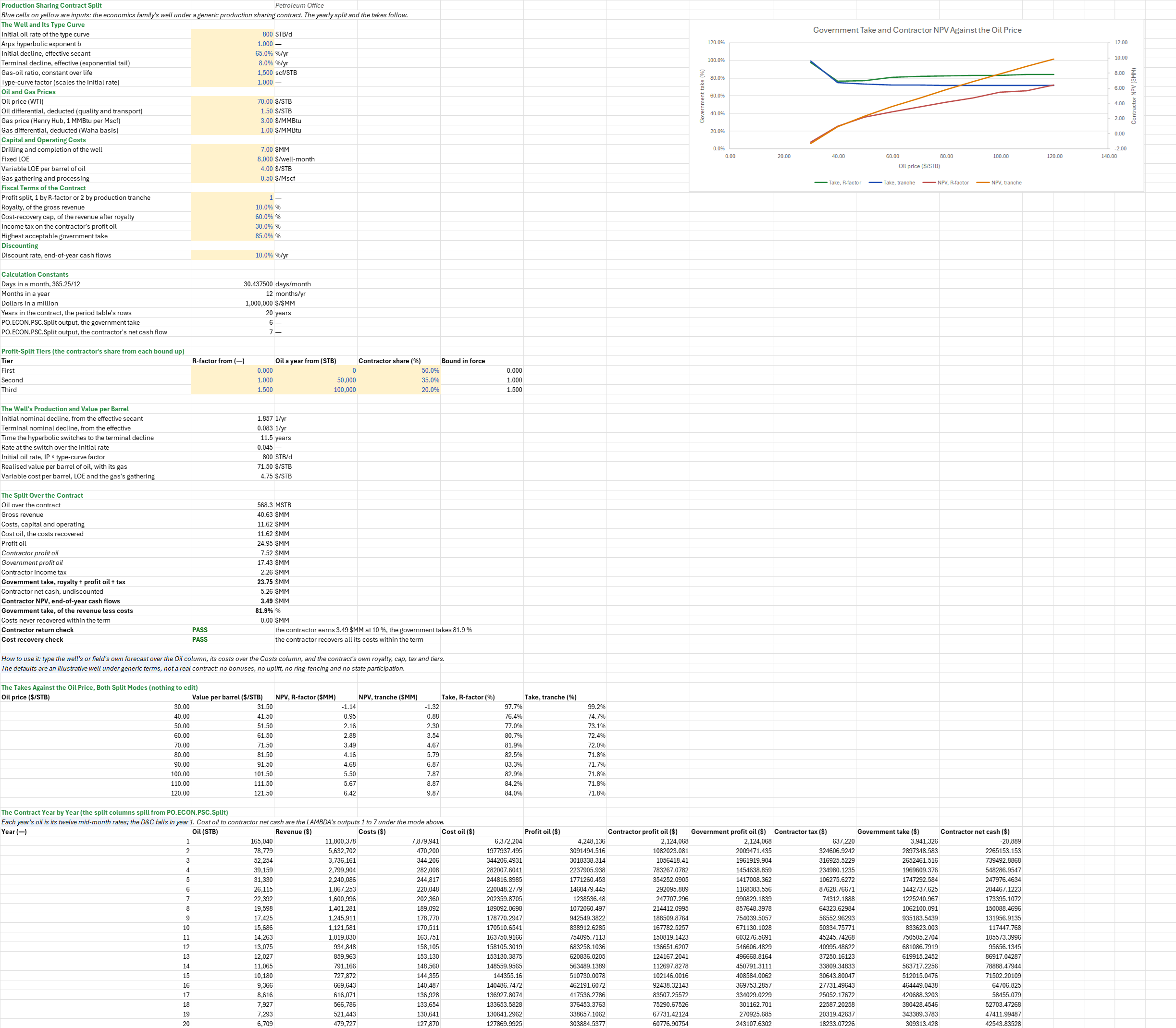
How does a production sharing contract divide a well's revenue, and what is left for the contractor? You enter the well's type curve, prices and costs and the contract's royalty, cost-recovery cap, income tax and profit-split tiers, by R-factor or by production tranche. You read off the royalty, cost oil, profit oil and tax year by year, the contract's totals, the government's take of the revenue less costs, and the contractor's NPV.
Parameters:
- The well: the type curve's initial rate
PSC_IP(STB/d), Arps exponentPSC_b, effective secant initial declinePSC_Deiand effective terminal declinePSC_Dterm, the gas-oil ratioPSC_GOR(scf/STB) and the type-curve factorPSC_TC - Prices: oil
PSC_Oil(/MMBtu) lessPSC_GasDiff, flat - Costs: the D&C
PSC_DC(/well-month), variable LOEPSC_LOEVar(/Mscf) - Fiscal terms: the split mode
PSC_Mode(1 by R-factor, 2 by production tranche), the royaltyPSC_Roy, the cost-recovery capPSC_CostCap(of the revenue after royalty), the income tax on the contractor's profit oilPSC_Taxand the highest acceptable government takePSC_TakeMax - Profit-split tiers (a table): each tier's R-factor lower bound
PSC_RfFrom, its yearly oil lower boundPSC_TrFrom(STB a year) and the contractor's sharePSC_Shares - Discounting: the discount rate
PSC_Disc, on end-of-year cash flows
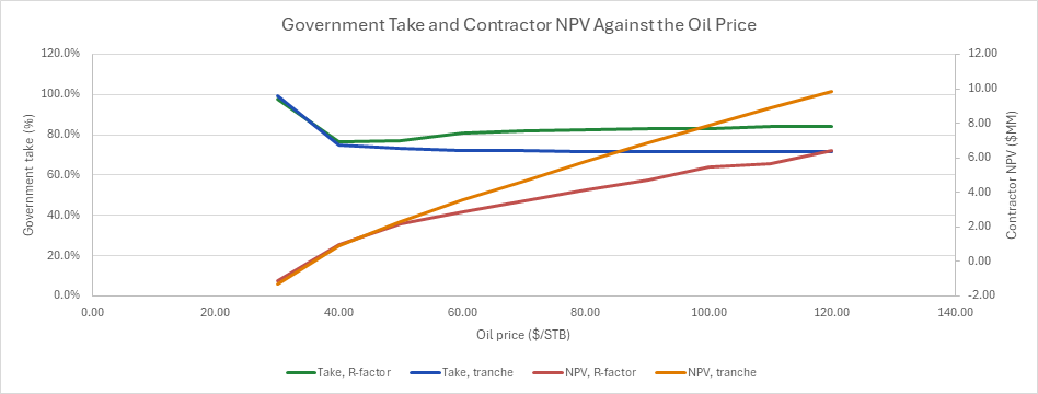
How to use it: The defaults are an illustrative well under generic terms, not a real contract. Type a field's own forecast over the Oil column and its costs over the Costs column, one row a year, and the contract's own royalty, cap, tax and tiers. Bonuses, an investment uplift, a domestic market obligation, ring-fencing and state participation are not in the split function: model them in cells around it. A sweep reprices the contract over the oil price under both modes, and the chart draws the government's take (left axis) and the contractor's NPV (right axis) against the oil price for each mode. The sheet flags a contractor that loses money, a government take above its limit, and costs never recovered within the term.
Method: Each year's oil is the sum of its twelve mid-month rates on the type curve times 30.4375 days. Its value per barrel is V = (Oil − OilDiff) + GOR/1000·(Gas − GasDiff), and its costs are the D&C in year 1 plus 12·LOE + (LOEVar + GOR/1000·Gath)·oil. The revenue is R = oil·V. The royalty is Roy·R and the net revenue N = R − royalty. The cumulative cost recovered is min(cumulative costs, last year's recovered + CostCap·N), so the cost oil is this year's step in it and the excess carries forward without uplift. The profit oil is N − cost oil. In mode 1 the contractor's share is that of the highest tier whose bound is at or below the R-factor, its cumulative receipts (cost oil plus its profit oil) over its cumulative costs to the end of the year before. In mode 2 each slice of the year's oil earns its tranche's share. The contractor's tax is Tax × its profit oil. The government takes the royalty, its profit oil and the tax. The contractor's net cash is cost oil + its profit oil − tax − costs, and its NPV discounts the year-k cash by (1 + Disc)^k. The government's take is its total over the revenue less costs.
Example: The default well is the economics family's (the well-program workbook's base case for one well, as on the One-Well NPV and IRR sheet): 800 STB/d initial on an Arps hyperbolic with b = 1 and a 65 %/yr effective secant decline switching to an 8 %/yr exponential tail, 1,500 scf/STB, $70/STB oil less $1.50 and $3.00/MMBtu gas less $1.00, a $7MM D&C, $8,000 a month of fixed LOE, $4/STB of variable LOE and $0.50/Mscf of gathering, over a 20-year contract. The fiscal terms are generic, after Johnston: a 10 % royalty, a 60 % cost-recovery cap, 30 % income tax, and the contractor's share of the profit oil falling from 50 % to 35 % at an R-factor of 1 and to 20 % at 1.5 (or, by tranche, at 50,000 and 100,000 STB a year). Cash is discounted at 10 %, and the government's take is held to 85 %.
In year 1 the well makes 165,040 STB, worth $11.80MM at $71.50 a barrel, oil and gas. The royalty takes $1.18MM, so the cap is 0.6 × 10.62 = $6.37MM, against $7.88MM of costs; $1.51MM carries into year 2. The $4.25MM of profit oil is split 50/50, since the R-factor is 0 in the first year, and the contractor's net cash is −$0.02MM. By year 2 the R-factor is (6.37 + 2.12)/7.88 = 1.08, so the contractor's share falls to 35 %. From year 5 it is 20 %, the R-factor having passed 1.5. Over 20 years the well makes 568.3 MSTB and $40.63MM of revenue against $11.62MM of costs, all recovered. The government takes $23.75MM: $4.06MM of royalty, $17.43MM of profit oil and $2.26MM of tax. That is 81.9 % of the $29.01MM of revenue less costs. The contractor nets $5.26MM, an NPV of $3.49MM at 10 %.
By tranche (mode 2) the contractor keeps more of the later, smaller years: its NPV is $4.67MM and the government's take 72.0 %. At $30 oil the cap leaves $1.95MM unrecovered and the contractor loses $1.14MM. The sweep shows the difference between the modes. Under the R-factor the take climbs from 76.4 % at $40 to 84.0 % at $120, and the contractor's NPV only from $0.95MM to $6.42MM. By tranche the take stays near 72 %, and the NPV rises from $0.88MM to $9.87MM.
Functions used
None: the blueprint calculates with Excel's own functions.
Names (63)
| Name | Refers to | Comment |
|---|---|---|
PO.ECON.PSC.SplitLAMBDA |
=LAMBDA(Mode, Gross, Price, Cost, Royalty, CostCap, Tax, Limits, Shares, Output, LET(rev, Gross*Price, roy, Royalty*rev, net, rev-roy, capv, CostCap*net, cumc, SCAN(0, Cost, LAMBDA(run_c, val_c, run_c+val_c)), cumcap, SCAN(0, capv, LAMBDA(run_k, val_k, run_k+val_k)), rec, cumcap+SCAN(0, cumc-cumcap, LAMBDA(low_r, val_r, MIN(low_r, val_r))), recprev, cumcap-capv+SCAN(0, cumc-Cost-cumcap+capv, LAMBDA(low_p, val_p, MIN(low_p, val_p))), costoil, rec-recprev, profit, net-costoil, tier, SCAN(0, Shares, LAMBDA(run_t, val_t, run_t+1)), ds, Shares-SCAN(0, tier, LAMBDA(run_d, tier_d, SUM((tier=tier_d-1)*Shares))), ix, SCAN(0, Gross, LAMBDA(run_i, val_i, run_i+1)), tranche, SCAN(0, ix, LAMBDA(run_q, per_q, LET(g, SUM((ix=per_q)*Gross), IF(g>0, SUM((g-Limits>0)*(g-Limits)*ds)/g, 0)))), receipts, SCAN(0, ix, LAMBDA(run_x, per_x, LET(cprev, SUM((ix<per_x)*Cost), rf, IF(cprev>0, run_x/cprev, 0), run_x+SUM((ix=per_x)*(costoil+SUM(ds*(rf>=Limits))*profit))))), back, SCAN(0, ix, LAMBDA(run_b, per_b, SUM((ix=per_b-1)*receipts))), cpo, CHOOSE(Mode, receipts-back-costoil, tranche*profit), gpo, profit-cpo, tx, Tax*cpo, govtake, roy+gpo+tx, ncf, costoil+cpo-tx-Cost, share, SCAN(0, govtake, LAMBDA(run_g, val_g, run_g+val_g))/SCAN(0, rev-Cost, LAMBDA(run_v, val_v, run_v+val_v)), CHOOSE(Output, costoil, profit, cpo, gpo, tx, govtake, ncf, share))) |
Production sharing contract split per period: cost oil under a cap with carry-forward, profit oil by R-factor (Mode 1) or production tranche (Mode 2), tax and takes |
PSC_IP |
$B$4 |
Initial oil rate of the type curve, STB/d |
PSC_b |
$B$5 |
Arps hyperbolic exponent b |
PSC_Dei |
$B$6 |
Initial decline, effective secant, %/yr |
PSC_Dterm |
$B$7 |
Terminal decline, effective (exponential tail), %/yr |
PSC_GOR |
$B$8 |
Gas-oil ratio, constant over life, scf/STB |
PSC_TC |
$B$9 |
Type-curve factor (scales the initial rate) |
PSC_Oil |
$B$11 |
Oil price (WTI), $/STB |
PSC_OilDiff |
$B$12 |
Oil differential, deducted (quality and transport), $/STB |
PSC_Gas |
$B$13 |
Gas price (Henry Hub, 1 MMBtu per Mscf), $/MMBtu |
PSC_GasDiff |
$B$14 |
Gas differential, deducted (Waha basis), $/MMBtu |
PSC_DC |
$B$16 |
Drilling and completion of the well, $MM |
PSC_LOE |
$B$17 |
Fixed LOE, $/well-month |
PSC_LOEVar |
$B$18 |
Variable LOE per barrel of oil, $/STB |
PSC_Gath |
$B$19 |
Gas gathering and processing, $/Mscf |
PSC_Mode |
$B$21 |
Profit split, 1 by R-factor or 2 by production tranche |
PSC_Roy |
$B$22 |
Royalty, of the gross revenue, % |
PSC_CostCap |
$B$23 |
Cost-recovery cap, of the revenue after royalty, % |
PSC_Tax |
$B$24 |
Income tax on the contractor's profit oil, % |
PSC_TakeMax |
$B$25 |
Highest acceptable government take, % |
PSC_Disc |
$B$27 |
Discount rate, end-of-year cash flows, %/yr |
PSC_Inputs |
$B$4:$B$27 |
The well's type curve, oil and gas prices, D&C and operating costs, the contract's split mode, royalty, cost-recovery cap, tax and the take limit, and the discount rate |
PSC_Days |
$B$30 |
Days in a month, 365.25/12, days/month |
PSC_MoYr |
$B$31 |
Months in a year, months/yr |
PSC_PerMM |
$B$32 |
Dollars in a million, $/$MM |
PSC_Years |
$B$33 |
Years in the contract, the period table's rows, years |
PSC_GovOut |
$B$34 |
PO.ECON.PSC.Split output, the government take |
PSC_CashOut |
$B$35 |
PO.ECON.PSC.Split output, the contractor's net cash flow |
PSC_Tiers |
$A$39:$E$41 |
Each tier's R-factor and yearly oil lower bounds, the contractor's share of the profit oil, and the bound the split mode uses |
PSC_RfFrom |
$B$39:$B$41 |
The tiers' R-factor lower bounds, ascending from 0 |
PSC_TrFrom |
$C$39:$C$41 |
The tiers' yearly oil lower bounds, ascending from 0, STB a year |
PSC_Shares |
$D$39:$D$41 |
The contractor's share of the profit oil in each tier |
PSC_Limits |
$E$39:$E$41 |
The tiers' lower bounds in force: R-factors in mode 1, yearly oil in mode 2 |
PSC_Di |
$B$44 |
Initial nominal decline, from the effective secant, 1/yr |
PSC_Dt |
$B$45 |
Terminal nominal decline, from the effective, 1/yr |
PSC_Ts |
$B$46 |
Time the hyperbolic switches to the terminal decline, years |
PSC_Qs |
$B$47 |
Rate at the switch over the initial rate |
PSC_Qi |
$B$48 |
Initial oil rate, IP × type-curve factor, STB/d |
PSC_Price |
$B$49 |
Realised value per barrel of oil, with its gas, $/STB |
PSC_OpexVar |
$B$50 |
Variable cost per barrel, LOE and the gas's gathering, $/STB |
PSC_OilTot |
$B$53 |
Oil over the contract, MSTB |
PSC_Revenue |
$B$54 |
Gross revenue, $MM |
PSC_Costs |
$B$55 |
Costs, capital and operating, $MM |
PSC_CostOil |
$B$56 |
Cost oil, the costs recovered, $MM |
PSC_ProfitOil |
$B$57 |
Profit oil, $MM |
PSC_CtrProfit |
$B$58 |
Contractor profit oil, $MM |
PSC_GovProfit |
$B$59 |
Government profit oil, $MM |
PSC_TaxPaid |
$B$60 |
Contractor income tax, $MM |
PSC_GovTake |
$B$61 |
Government take, royalty + profit oil + tax, $MM |
PSC_CtrCash |
$B$62 |
Contractor net cash, undiscounted, $MM |
PSC_CtrNPV |
$B$63 |
Contractor NPV, end-of-year cash flows, $MM |
PSC_GovShare |
$B$64 |
Government take, of the revenue less costs, % |
PSC_Unrecovered |
$B$65 |
Costs never recovered within the term, $MM |
PSC_ReturnCheck |
$B$66 |
Contractor return check verdict |
PSC_ReturnCheckNote |
$C$66 |
Contractor return check comment |
PSC_RecoveryCheck |
$B$67 |
Cost recovery check verdict |
PSC_RecoveryCheckNote |
$C$67 |
Cost recovery check comment |
PSC_Results |
$B$44:$B$67 |
The decline terms, the value and variable cost per barrel, the contract's revenue, costs, cost oil, profit oil, tax and takes, the contractor's cash and NPV, and two checks |
PSC_Sweep |
$A$74:$F$83 |
Oil prices, the value per barrel at each, and the contractor's NPV and the government's take by R-factor and by tranche |
PSC_Gross |
$B$88:$B$107 |
The contract's oil, one row a year, STB |
PSC_Cost |
$D$88:$D$107 |
The contract's recoverable costs, capital and operating, one row a year, $ |
PSC_Contract |
$A$88:$D$107 |
Each contract year, its oil, its gross revenue and its recoverable costs |
PSC_SweepCurve |
$A$74:$F$83 |
Government Take and Contractor NPV Against the Oil Price |
Details
| Inserts | 107 rows × 11 columns |
| Category | Petroleum Economics |
| For agents and tools | Descriptor (.md) |