Interference and Pulse Test
Description
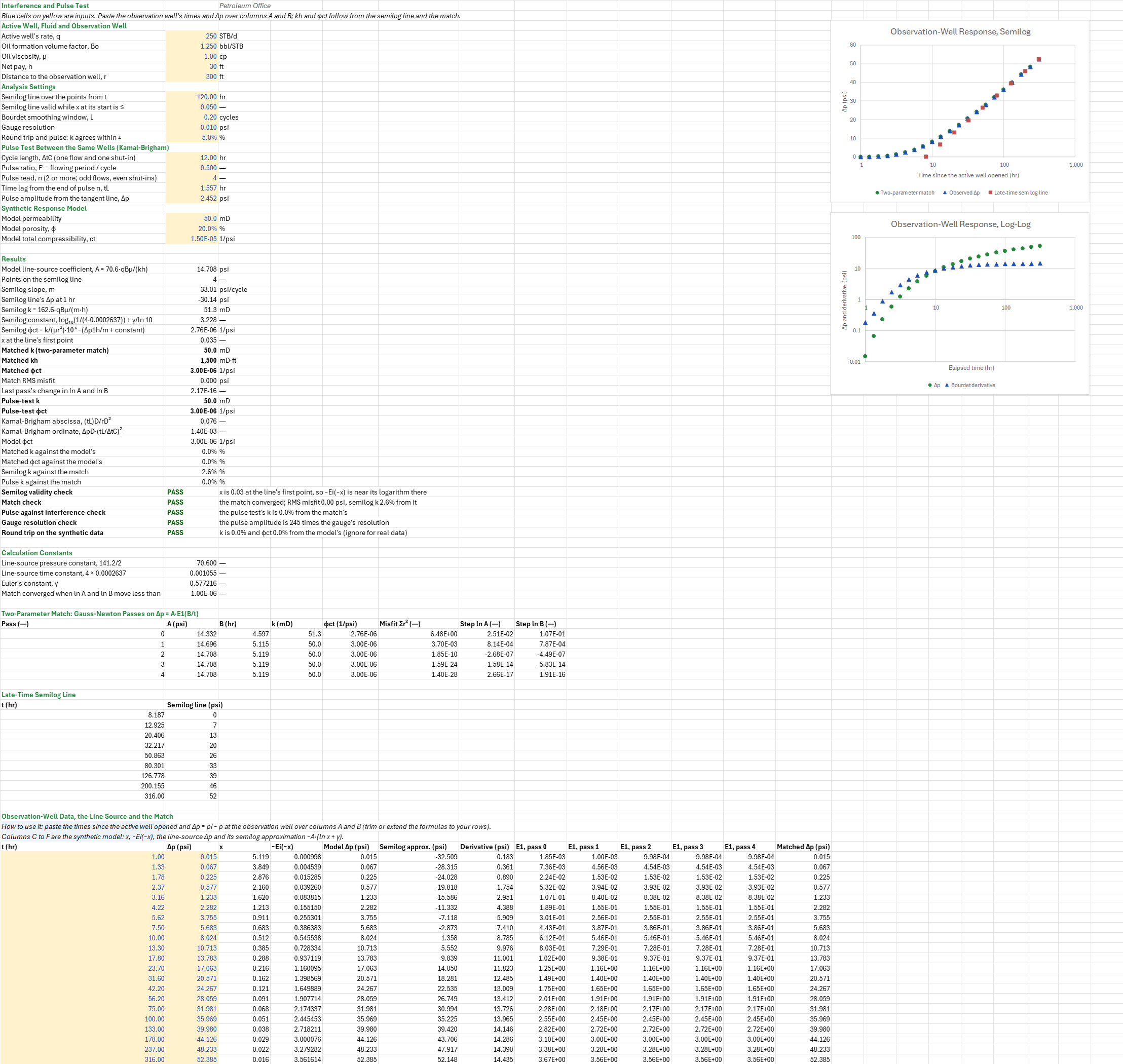
What interwell permeability-thickness kh and storativity φct does an interference test give, and does a pulse test between the same two wells agree? You paste the observation well's times and pressure drop, and set the active well's rate, the fluid, h, the well spacing and one pulse's lag and amplitude. The sheet reads the drop on the line-source solution at the observation well, from its late-time semilog line and from a match of the whole curve. You read off kh, k and φct from each, and from the pulse.
Parameters:
- Active well, fluid and spacing: the rate, Bo, μ, h and the distance to the observation well (
IT_q,IT_Bo,IT_mu,IT_h,IT_r) - Analysis settings: where the semilog line starts (
IT_From), the x it must be below there (IT_xMax, 0.05), the Bourdet window (IT_L), the gauge's resolution (IT_Res) and the agreement tolerance (IT_KTol, ±5 %) - Pulse test: the cycle length, pulse ratio, pulse number, time lag and amplitude (
IT_dtC,IT_Fp,IT_n,IT_tL,IT_PDp) - Synthetic model: k, φ and ct (
IT_ModelK,IT_phi,IT_ct) - Data: time and Δp at the observation well, the region
IT_Data
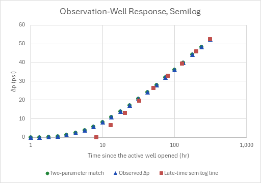
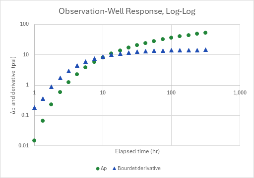
How to use it: Paste the times since the active well opened and the observation well's Δp = pi − p over columns A and B, and set the rate, the fluid, h and r. Remove the trend before you take Δp. Read the pulse's lag and amplitude off the observation gauge after drift correction, as the pulse analysis defines them: the lag from the end of pulse n to its extremum, and the amplitude from the line tangent to the two neighbouring extrema. The model columns and the round-trip check then don't apply. A semilog plot draws the observed Δp, the match and the semilog line, and a log-log plot draws Δp and its Bourdet derivative.
Method: One well produces at a constant rate. An observation well a distance r away records the small pressure drop that reaches it. In an infinite, homogeneous reservoir that drop is the line-source solution, Δp = −70.6·qBμ/(kh)·Ei(−x) with x = φμct·r²/(4·0.0002637·k·t). The sheet draws it with the exponential integral beside its late-time logarithm, −Ei(−x) ≈ −ln x − γ, so you can see where the semilog line holds.
- Semilog line. The line is fitted by least squares over the points from the line's start time. Its slope m gives k = 162.6·qBμ/(m·h). Its Δp at 1 hr gives φct = k/(μr²)·10^−(Δp1h/m + log₁₀(1/(4·0.0002637)) + γ/ln 10), the line-source form of the MDH skin equation at zero skin. The line holds once x is small. The sheet reports x at the line's first point and warns above the x limit.
- Match. The match fits Δp = A·E1(B/t) to every point, with A = 70.6·qBμ/(kh) and B = φμct·r²/(4·0.0002637·k). It works in ln A and ln B. The sensitivities are A·E1(B/t) and −A·e^(−B/t), because the derivative of E1(x) is −e^(−x)/x. Each Gauss-Newton pass therefore needs one column of E1 values and five sums. It starts from the semilog line and takes four passes, each written out as its own columns, so the sheet holds no circular reference. Then k = 70.6·qBμ/(A·h) and φct = B·4·0.0002637·k/(μr²).
- Pulse test. The pulse analysis (Kamal and Brigham) finds the diffusivity whose line-source pulse train has the measured lag, then reads k from the amplitude. Odd pulses are flow periods and even pulses shut-ins.
Example: The PTA reference well (250 STB/d, Bo 1.25 bbl/STB, μ 1 cp, h 30 ft) produces into the buildup sheets' reservoir (k 50 mD, φ 20 %, ct 1.5 × 10⁻⁵ 1/psi, so φct = 3 × 10⁻⁶ 1/psi). The observation well is 300 ft away, read from 1 to 316 hr. The drop reaches 0.015 psi at 1 hr and 52.4 psi at 316 hr.
The semilog line over the 4 points from 133 hr has m = 33.01 psi/cycle and crosses Δp = 0 near 8.2 hr, so k = 51.31 mD and φct = 2.764 × 10⁻⁶ 1/psi, 2.6 % high and 7.9 % low. x is 0.035 at 133 hr, under the 0.05 limit: the line is close, but even there −Ei(−x) has not quite reached its logarithm. The match starts from that line and lands on k = 50.00 mD, kh = 1,500 md·ft and φct = 3.000 × 10⁻⁶ 1/psi. The first pass takes it to 50.04 mD, the second to within 10⁻⁶, and the third and fourth change nothing. The pulse test runs 6-hour pulses, a 12-hour cycle at F′ = ½, between the same wells. Pulse 4, a shut-in, lags 1.5571 hr behind its end with an amplitude of 2.4515 psi, which gives k = 50.00 mD and φct = 3.000 × 10⁻⁶ 1/psi. On Kamal and Brigham's chart that is (tL)D/rD² = 0.0760 and ΔpD·(tL/ΔtC)² = 0.00140. The amplitude is 245 times the 0.01 psi gauge resolution.
The sheet was checked against the Engineering library's interference-test pressure drop (Team76.Engineering 6.0.0), the line-source drop at the observation well, on the same well, fluid, rock, rate and 21 times. The sheet's Δp column (the exponential integral with 141.2/2 and 4 × 0.0002637) equals it to 10⁻⁶ psi at every time. A standalone script then repeats the analysis on the library's Δp. It fits the semilog line with its own least squares and runs its own Gauss-Newton with its own E1 (power series and continued fraction, not the add-in's exponential integral), to convergence rather than four passes. A brute-force grid over k and φct finds the same minimum. It reproduces m 33.0087, k 51.3122, φct 2.76429 × 10⁻⁶ and x 0.0345607, every pass of the match to 10⁻⁶, and the converged k = 50 and φct = 3 × 10⁻⁶. The pulse readings come from the independent pulse forward model of the pulse analysis's own reference checks (line source, extrema by bisection, the tangent line by golden-section search). At the extremum, its pressure agrees with the library's interference-test pressure drop over the pulse train's rate history to 10⁻¹⁴ psi. No printed interference or pulse example with every input given was to hand (Earlougher's chapter 9 examples were not), so the sheet is not compared with a published one.
Functions used
PO.PTA.Horner.k(m, q, B, Ul, h)
Calculates permeability from the semilog slope of a buildup or drawdown, k = 162.6·q·B·Ul/(abs(m)·h), [mD].
PO.Math.Ei(x)
Calculates the exponential integral function Ei(x).
PO.DCA.Diag.Bourdet.SemiLog(x_values, y_values, t, L)
Calculates the classical Bourdet derivative dy/d(ln x) at point t, the log-domain estimator used for semilog and log-log well-test analysis. Multiply by LN(10) for a slope per log cycle.
Names (61)
| Name | Refers to | Comment |
|---|---|---|
PO.PTA.Pulse.AnalysisLAMBDA |
=LAMBDA(tL, dp, dtC, Fp, n, q, B, mu, h, robs, output, IF(OR(n<2, n<>ROUND(n, 0), Fp<=0, Fp>=1, tL<=0, dp<=0, dtC<=0), NA(), LET(lam, tL/dtC, nn, 600, jc, SEQUENCE(n+2, 1, 0), xs, jc/2+(Fp-0.5)*(1-(-1)^jc)/2, sgc, (-1)^jc, sgn, (-1)^(n+1), xepv, (n-1)/2+(Fp-0.5)*(1-(-1)^(n-1))/2, xen, n/2+(Fp-0.5)*(1-(-1)^n)/2, xenx, (n+1)/2+(Fp-0.5)*(1-(-1)^(n+1))/2, xenn, (n+2)/2+(Fp-0.5)*(1-(-1)^(n+2))/2, ig, SEQUENCE(nn+1, 1, 0), wz, xenx-xen, dz, xen+wz*ig/nn-TRANSPOSE(xs), pos, (dz>0)*1, dzc, pos*dz+1-pos, lgc, REDUCE(-9, SEQUENCE(121), LAMBDA(acc, i, IF(acc>-9, acc, LET(aa, 10^(-3.05+0.05*i), dv, MMULT(pos*EXP(-aa/(4*dzc))/dzc, sgc), cnt, SUM((dv*sgn>0)*1), da, SUM((ig=cnt-1)*dv), db, SUM((ig=cnt)*dv), lagx, IF(OR(cnt=0, cnt>nn), 2, wz*(cnt-1+da/(da-db))/nn), IF(lagx>=lam, -3.05+0.05*i, -9))))), lg, REDUCE(lgc-0.05, SEQUENCE(30), LAMBDA(acc, i, LET(aa, 10^(acc+0.05/2^i), dv, MMULT(pos*EXP(-aa/(4*dzc))/dzc, sgc), cnt, SUM((dv*sgn>0)*1), da, SUM((ig=cnt-1)*dv), db, SUM((ig=cnt)*dv), lagx, IF(OR(cnt=0, cnt>nn), 2, wz*(cnt-1+da/(da-db))/nn), acc+IF(lagx<lam, 0.05/2^i, 0)))), la, 10^lg, lagf, LET(aa, la, dv, MMULT(pos*EXP(-aa/(4*dzc))/dzc, sgc), cnt, SUM((dv*sgn>0)*1), da, SUM((ig=cnt-1)*dv), db, SUM((ig=cnt)*dv), lagx, IF(OR(cnt=0, cnt>nn), 2, wz*(cnt-1+da/(da-db))/nn), lagx), ik, SEQUENCE(2*nn+1), inw, (ik<=nn)*1, inx, (ik>nn)*(ik<=2*nn), atc, (ik>2*nn)*1, gx, inw*(xepv+(xen-xepv)*ik/nn)+inx*(xenx+(xenn-xenx)*(ik-nn)/nn)+atc*(xen+lam), dx, gx-TRANSPOSE(xs), px, (dx>0)*1, zx, la/(4*(px*dx+1-px)), lo, (zx<=1)*1, eone, lo*(-LN(zx)-0.57721566+zx*(0.99999193+zx*(-0.24991055+zx*(0.05519968+zx*(-0.00976004+zx*0.00107857)))))+(1-lo)*EXP(0-zx)/zx*(zx^4+8.5733287401*zx^3+18.059016973*zx^2+8.6347608925*zx+0.2677737343)/(zx^4+9.5733223454*zx^3+25.6329561486*zx^2+21.0996530827*zx+3.9584969228), pdx, MMULT(px*eone, sgc)/2, big, 10^300, sl, REDUCE(0, SEQUENCE(60), LAMBDA(acc, i, LET(v, sgn*(pdx-acc*gx), f, MIN(v+(1-inw)*big)-MIN(v+(1-inx)*big), acc+IF(sgn*f<0, 1, -1)*100/2^i))), base, sgn*MIN(sgn*(pdx-sl*gx)+(1-inw)*big), ad, ABS(SUM(atc*pdx)-base-sl*(xen+lam)), perm, 141.2*q*B*mu*ad/(h*dp), IF(OR(lgc<-2.99, ABS(lagf-lam)>0.0001*lam), NA(), IF(output="k", perm, IF(output="phict", 0.0002637*perm*la*dtC/(mu*robs^2), IF(output="tLD", lam/la, IF(output="dpD", ad*lam^2, NA())))))))) |
Kamal-Brigham pulse test from the time lag and amplitude of pulse n (≥ 2) on the line-source response; output "k" [md], "phict" [1/psi], "tLD" (tL)D/rD² or "dpD" ΔpD·(tL/ΔtC)², the chart ordinates. |
IT_q |
$B$4 |
Active well's rate, q, STB/d |
IT_Bo |
$B$5 |
Oil formation volume factor, Bo, bbl/STB |
IT_mu |
$B$6 |
Oil viscosity, μ, cp |
IT_h |
$B$7 |
Net pay, h, ft |
IT_r |
$B$8 |
Distance to the observation well, r, ft |
IT_From |
$B$10 |
Semilog line over the points from t, hr |
IT_xMax |
$B$11 |
Semilog line valid while x at its start is ≤ |
IT_L |
$B$12 |
Bourdet smoothing window, L, cycles |
IT_Res |
$B$13 |
Gauge resolution, psi |
IT_KTol |
$B$14 |
Round trip and pulse: k agrees within ±, % |
IT_dtC |
$B$16 |
Cycle length, ΔtC (one flow and one shut-in), hr |
IT_Fp |
$B$17 |
Pulse ratio, F′ = flowing period / cycle |
IT_n |
$B$18 |
Pulse read, n (2 or more; odd flows, even shut-ins) |
IT_tL |
$B$19 |
Time lag from the end of pulse n, tL, hr |
IT_PDp |
$B$20 |
Pulse amplitude from the tangent line, Δp, psi |
IT_ModelK |
$B$22 |
Model permeability, mD |
IT_phi |
$B$23 |
Model porosity, φ, % |
IT_ct |
$B$24 |
Model total compressibility, ct, 1/psi |
IT_Inputs |
$B$4:$B$24 |
The active well's rate, the fluid, h and the well spacing, the semilog window, the gauge, the pulse readings and the synthetic model |
IT_AModel |
$B$27 |
Model line-source coefficient, A = 70.6·qBμ/(kh), psi |
IT_NSl |
$B$28 |
Points on the semilog line |
IT_M |
$B$29 |
Semilog slope, m, psi/cycle |
IT_Dp1h |
$B$30 |
Semilog line's Δp at 1 hr, psi |
IT_KSl |
$B$31 |
Semilog k = 162.6·qBμ/(m·h), mD |
IT_LsC |
$B$32 |
Semilog constant, log₁₀(1/(4·0.0002637)) + γ/ln 10 |
IT_PhictSl |
$B$33 |
Semilog φct = k/(μr²)·10^−(Δp1h/m + constant), 1/psi |
IT_XFrom |
$B$34 |
x at the line's first point |
IT_K |
$B$35 |
Matched k (two-parameter match), mD |
IT_Kh |
$B$36 |
Matched kh, mD·ft |
IT_Phict |
$B$37 |
Matched φct, 1/psi |
IT_Rms |
$B$38 |
Match RMS misfit, psi |
IT_Conv |
$B$39 |
Last pass's change in ln A and ln B |
IT_KPulse |
$B$40 |
Pulse-test k, mD |
IT_PhictPulse |
$B$41 |
Pulse-test φct, 1/psi |
IT_TLD |
$B$42 |
Kamal-Brigham abscissa, (tL)D/rD² |
IT_DpD |
$B$43 |
Kamal-Brigham ordinate, ΔpD·(tL/ΔtC)² |
IT_PhictModel |
$B$44 |
Model φct, 1/psi |
IT_KErr |
$B$45 |
Matched k against the model's, % |
IT_PErr |
$B$46 |
Matched φct against the model's, % |
IT_SlErr |
$B$47 |
Semilog k against the match, % |
IT_PulseErr |
$B$48 |
Pulse k against the match, % |
IT_SemilogCheck |
$B$49 |
Semilog validity check verdict |
IT_SemilogCheckNote |
$C$49 |
Semilog validity check comment |
IT_MatchCheck |
$B$50 |
Match check verdict |
IT_MatchCheckNote |
$C$50 |
Match check comment |
IT_PulseCheck |
$B$51 |
Pulse against interference check verdict |
IT_PulseCheckNote |
$C$51 |
Pulse against interference check comment |
IT_GaugeCheck |
$B$52 |
Gauge resolution check verdict |
IT_GaugeCheckNote |
$C$52 |
Gauge resolution check comment |
IT_TripCheck |
$B$53 |
Round trip on the synthetic data verdict |
IT_TripCheckNote |
$C$53 |
Round trip on the synthetic data comment |
IT_Results |
$B$27:$B$53 |
The semilog line, k and φct from it, the match's k, kh and φct, the pulse test's k and φct, the round trip and the checks |
IT_cP |
$B$56 |
Line-source pressure constant, 141.2/2 |
IT_cX |
$B$57 |
Line-source time constant, 4 × 0.0002637 |
IT_Euler |
$B$58 |
Euler's constant, γ |
IT_ConvTol |
$B$59 |
Match converged when ln A and ln B move less than |
IT_Passes |
$A$63:$H$67 |
The match's passes: A and B, the k and φct they give, the misfit and the Gauss-Newton step |
IT_Data |
$A$85:$B$105 |
Time and the observation well's Δp (the synthetic model's until you paste a gauge's) |
IT_Analysis |
$C$85:$M$105 |
Per row: the model's x, −Ei(−x), Δp and semilog approximation, the Bourdet derivative, the E1 column of each match pass, and the matched Δp |
IT_Curve |
$A$85:$M$105 |
Observation-Well Response, Semilog |
Details
| Inserts | 105 rows × 13 columns |
| Category | Pressure Transient Analysis |
| For agents and tools | Descriptor (.md) |