Injection Falloff and Step-Rate Test
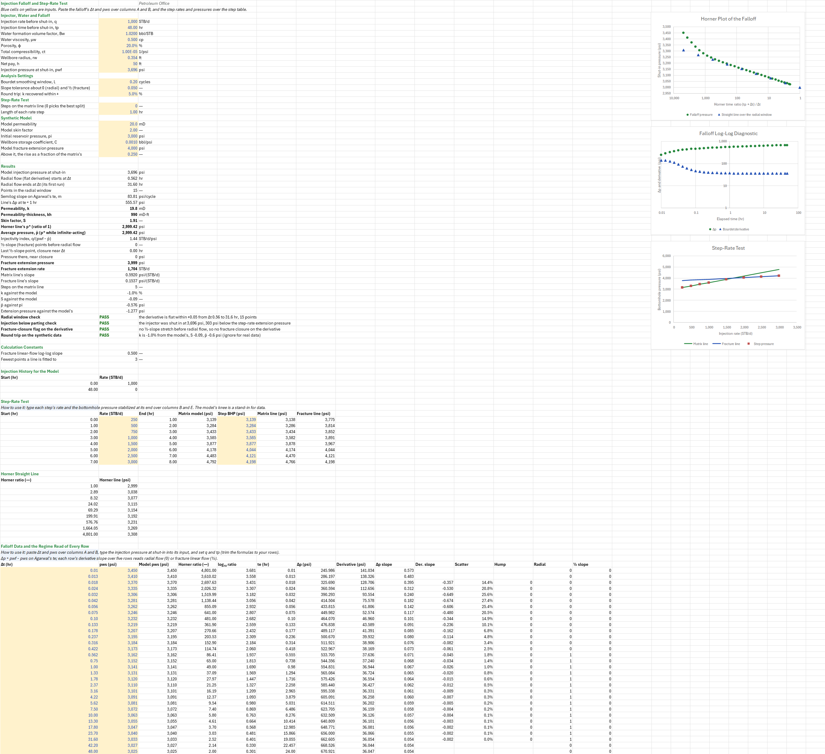
Description
What kh, skin and average pressure does a water injector's falloff give, and was the well injecting below parting pressure? You paste the falloff's shut-in times and pressures, the injection rate, time and pressure at shut-in, and each step-rate step's rate and stabilized pressure. The sheet finds the radial-flow window from the Bourdet derivative, fits the MDH and Horner lines inside it, and fits the step-rate test's two lines. You read off k, kh, skin, p*, the injectivity and the fracture extension pressure and rate.
Parameters:
- Injector, water and falloff: the injection rate and time, Bw, μw, φ, ct, rw, h, and the injection pressure at shut-in (
FO_q,FO_tp,FO_Bw,FO_mu,FO_phi,FO_ct,FO_rw,FO_h,FO_Pwf, which takes the model's) - Analysis settings: the Bourdet window (
FO_L), the slope tolerance about 0 and ½ (FO_Tol, ±0.05), and the round-trip tolerance on k (FO_KTol, ±5 %) - Step-rate test: the steps on the matrix line (
FO_nlow, 0 picks the best split) and the step length (FO_StepHr) - Synthetic model: k, skin, pi, C, the extension pressure and the fracture's share of the rise above it (
FO_ModelK,FO_ModelS,FO_Pi,FO_C,FO_ModelPfe,FO_Frac) - Data: the falloff's Δt and pws, the region
FO_Data, and the steps' rates and pressures, the regionsFO_StepsandFO_StepFit
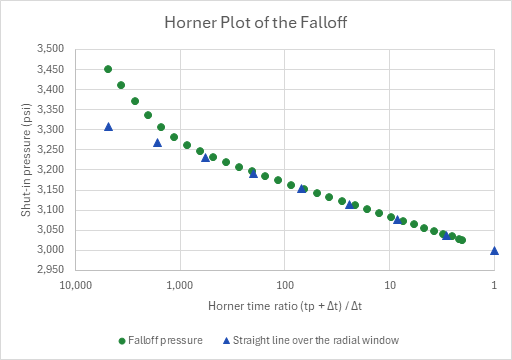
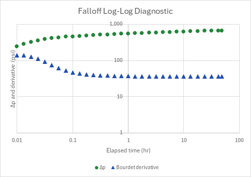
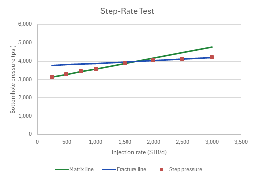
How to use it: Paste the falloff's Δt and pws over columns A and B, type the injection pressure at shut-in over the model's, and set q and tp. With a varying injection rate, use tp = cumulative injection × 24/q at the last rate. Type each step's rate and stabilized bottomhole pressure over the step table's Rate and Step BHP columns. The model columns and the round-trip check then don't apply. A Horner plot, a log-log plot of Δp and its derivative, and the step-rate plot with both lines are drawn.
Method: After injecting at a constant rate for tp hours the well is shut in, and its bottomhole pressure falls back towards the reservoir's. The sheet reads Δp = pwf − pws against Agarwal's equivalent time te = tp·Δt/(tp + Δt).
- Derivative and regimes. te = tp/R, where R = (tp + Δt)/Δt is the Horner ratio. The derivative is Bourdet's dΔp/d ln te with window L. Each interior row gets the derivative's log-log slope over the five rows centred on it (the least-squares slope of ln derivative on ln te), the scatter of those five derivatives, and a storage-hump flag. A row is radial when its slope is within ±Tol of 0, its scatter is under Tol/2 and it is not on the hump. It is a fracture row when both the derivative's slope and Δp's own (derivative ÷ Δp) are within ±Tol of ½. The radial window is the first unbroken run of radial rows. A ½ slope before radial flow is a fracture's linear flow, so the sheet flags it and reads where it ends, near closure.
- Lines. Over the window, the MDH fit puts Δp against log₁₀ te: k = 162.6·qBμ/(m·h) and S = 1.151·[Δp1h/m − log₁₀(k/(φμct·rw²)) + 3.23]. The same points of pws against log₁₀ R give the Horner line, whose intercept at R = 1 is p*. For a new injector in an infinite-acting reservoir the average pressure is p*. The injectivity index is q/(pwf − p̄).
- Step-rate test. The step-rate fit puts least-squares lines through the steps below and above the break and returns their crossing, the extension pressure and rate. With the matrix-line step count at 0 it tries every split and keeps the one of least squared error. The injection pressure at shut-in is checked against the extension pressure.
Example: A water injector takes 1,000 STB/d for 48 hr (Bw 1.02, μw 0.5 cp) into k 20 mD, h 50 ft, φ 20 %, ct 10⁻⁵ 1/psi, with skin 2 and a liquid-filled wellbore's storage of 0.001 bbl/psi, at pi 3,000 psi. The vertical-well model on the injection rate puts the injection pressure at 3,695.89 psi. The falloff is read from 0.01 to 48 hr. The storage hump peaks before the first reading. The derivative falls to its plateau of about 36 psi, flat within ±0.05 from Δt = 0.562 to 31.6 hr, 15 points. The MDH line there has m = 83.81 psi/cycle, so k = 19.79 mD (kh 990 md·ft) and S = 1.91, 1.0 % and 0.09 below the model's, within ±5 %. p* = 2,999.42 psi, 0.58 psi under pi, and the injectivity is 1.44 STB/d/psi. No ½-slope rows appear: the injector isn't fractured.
The step-rate test runs eight 1-hour steps from 250 to 3,000 STB/d on the same well. Each step's pressure is the model's at the step's end. Above a model extension pressure of 4,000 psi the open fracture takes the extra rate, and the pressure rises only a quarter as fast. The automatic split keeps 5 steps on the matrix line (slope 0.592 psi per STB/d) and 3 on the fracture line (0.154). They cross at 1,704 STB/d and 3,998.72 psi, 1.3 psi under the model's. The injection pressure is 303 psi below it, so the well was injecting below parting pressure.
The sheet was checked against the Engineering library's falloff pressure excess (Team76.Engineering 6.0.0) on the same model, rate, injection time and 31 shut-in times. The sheet's pws minus pi equals it to 10⁻⁵ psi. A standalone script then repeats the analysis. It takes the library's semilog Bourdet derivative and applies the sheet's slope, scatter and hump rule in its own code. It fits the window with its own least squares and gets k and S from the library's buildup permeability-from-slope and Horner skin. It reproduces the window (0.562 to 31.6 hr, 15 points), m 83.8059, k 19.79, S 1.91156 and p* 2,999.42. For the step-rate test the script computes each step's matrix pressure with the library's PTA pressure drop on the step history, applies the knee, and fits every split by its own least squares. It reproduces the split of 5, 3,998.72 psi, 1,703.99 STB/d and both slopes. The same script gives the skin-5 case. No printed falloff or step-rate example with every input given was to hand, so the sheet is not compared with a published one.
Functions used
PO.PTA.Pw.VW(time, prod_data, B, Ul, C, Rw, S, Ct, porosity, h, K)
Calculates wellbore pressure drop for vertical well in infinite homogeneous reservoir, [psi].
PO.PTA.Horner.Ratio(tp, dt)
Calculates the Horner time ratio (tp + dt)/dt, the x-axis of a Horner plot, [dimensionless].
PO.DCA.Diag.Bourdet.SemiLog(x_values, y_values, t, L)
Calculates the classical Bourdet derivative dy/d(ln x) at point t, the log-domain estimator used for semilog and log-log well-test analysis. Multiply by LN(10) for a slope per log cycle.
Names (64)
| Name | Refers to | Comment |
|---|---|---|
PO.PTA.MDH.FitLAMBDA |
=LAMBDA(t, dp, q, B, mu, h, phi, ct, rw, output, LET(x, LOG10(t), m, SLOPE(dp, x), dp_1h, INTERCEPT(dp, x), perm, 162.6*q*B*mu/(m*h), skin, 1.151*(dp_1h/m-LOG10(perm/(phi*mu*ct*rw^2))+3.23), IF(m<=0, NA(), IF(output="k", perm, IF(output="S", skin, IF(output="m", m, IF(output="dp1h", dp_1h, NA()))))))) |
MDH semilog straight-line fit of a drawdown: least squares of Δp against log10(t) over the points given; output "k" [mD], "S" [dimensionless], "m" [psi/cycle] or "dp1h" [psi], the line's Δp at 1 h. |
PO.PTA.StepRate.FitLAMBDA |
=LAMBDA(q, p, nlow, output, LET(cnt, ROWS(q), qa, AVERAGE(q), pa, AVERAGE(p), qc, q-qa, pc, p-pa, ix, SEQUENCE(cnt), kk, SEQUENCE(cnt-3, 1, 2), msk, --(TRANSPOSE(ix)<=kk), nlo, kk, nhi, cnt-kk, sxlo, MMULT(msk, qc), sylo, MMULT(msk, pc), sxxlo, MMULT(msk, qc^2), sxylo, MMULT(msk, qc*pc), syylo, MMULT(msk, pc^2), sxhi, SUM(qc)-sxlo, syhi, SUM(pc)-sylo, sxxhi, SUM(qc^2)-sxxlo, sxyhi, SUM(qc*pc)-sxylo, syyhi, SUM(pc^2)-syylo, cxxlo, sxxlo-sxlo^2/nlo, cxylo, sxylo-sxlo*sylo/nlo, cxxhi, sxxhi-sxhi^2/nhi, cxyhi, sxyhi-sxhi*syhi/nhi, sse, syylo-sylo^2/nlo-cxylo^2/cxxlo+syyhi-syhi^2/nhi-cxyhi^2/cxxhi, pick, IF(nlow>0, nlow, MIN(IF(sse=MIN(sse), kk, cnt))), sel, --(kk=pick), slo, SUM(sel*cxylo/cxxlo), shi, SUM(sel*cxyhi/cxxhi), ilo, SUM(sel*(sylo-slo*sxlo)/nlo), ihi, SUM(sel*(syhi-shi*sxhi)/nhi), qx, IF(slo>shi, (ihi-ilo)/(slo-shi), 0), IF(OR(cnt<5, nlow<0, nlow=1, nlow>cnt-2, slo<=shi), NA(), IF(output="p", pa+ilo+slo*qx, IF(output="q", qa+qx, IF(output="mlo", slo, IF(output="mhi", shi, IF(output="n", pick, NA())))))))) |
Two-line step-rate test fit: least squares of the matrix and the fracture lines, split at nlow points (0 picks the split of least total squared error); output "p" extension pressure, "q" extension rate, "mlo", "mhi" slopes or "n" split. |
FO_q |
$B$4 |
Injection rate before shut-in, q, STB/d |
FO_tp |
$B$5 |
Injection time before shut-in, tp, hr |
FO_Bw |
$B$6 |
Water formation volume factor, Bw, bbl/STB |
FO_mu |
$B$7 |
Water viscosity, μw, cp |
FO_phi |
$B$8 |
Porosity, φ, % |
FO_ct |
$B$9 |
Total compressibility, ct, 1/psi |
FO_rw |
$B$10 |
Wellbore radius, rw, ft |
FO_h |
$B$11 |
Net pay, h, ft |
FO_Pwf |
$B$12 |
Injection pressure at shut-in, pwf, psi |
FO_L |
$B$14 |
Bourdet smoothing window, L, cycles |
FO_Tol |
$B$15 |
Slope tolerance about 0 (radial) and ½ (fracture) |
FO_KTol |
$B$16 |
Round trip: k recovered within ±, % |
FO_nlow |
$B$18 |
Steps on the matrix line (0 picks the best split) |
FO_StepHr |
$B$19 |
Length of each rate step, hr |
FO_ModelK |
$B$21 |
Model permeability, mD |
FO_ModelS |
$B$22 |
Model skin factor |
FO_Pi |
$B$23 |
Initial reservoir pressure, pi, psi |
FO_C |
$B$24 |
Wellbore storage coefficient, C, bbl/psi |
FO_ModelPfe |
$B$25 |
Model fracture extension pressure, psi |
FO_Frac |
$B$26 |
Above it, the rise as a fraction of the matrix's |
FO_Inputs |
$B$4:$B$26 |
Rate, injection time, water and rock, the pressure at shut-in, the window settings, the step-rate split and step length, and the synthetic model |
FO_PwfModel |
$B$29 |
Model injection pressure at shut-in, psi |
FO_RadStart |
$B$30 |
Radial flow (flat derivative) starts at Δt, hr |
FO_RadEnd |
$B$31 |
Radial flow ends at Δt (its first run), hr |
FO_NRad |
$B$32 |
Points in the radial window |
FO_M |
$B$33 |
Semilog slope on Agarwal's te, m, psi/cycle |
FO_Dp1h |
$B$34 |
Line's Δp at te = 1 hr, psi |
FO_K |
$B$35 |
Permeability, k, mD |
FO_Kh |
$B$36 |
Permeability-thickness, kh, mD·ft |
FO_S |
$B$37 |
Skin factor, S |
FO_Pstar |
$B$38 |
Horner line's p* (ratio of 1), psi |
FO_Pavg |
$B$39 |
Average pressure, p̄ (p* while infinite-acting), psi |
FO_II |
$B$40 |
Injectivity index, q/(pwf − p̄), STB/d/psi |
FO_NHalf |
$B$41 |
½-slope (fracture) points before radial flow |
FO_TClose |
$B$42 |
Last ½-slope point, closure near Δt, hr |
FO_PClose |
$B$43 |
Pressure there, near closure, psi |
FO_Pfe |
$B$44 |
Fracture extension pressure, psi |
FO_Qfe |
$B$45 |
Fracture extension rate, STB/d |
FO_MLo |
$B$46 |
Matrix line's slope, psi/(STB/d) |
FO_MHi |
$B$47 |
Fracture line's slope, psi/(STB/d) |
FO_NLo |
$B$48 |
Steps on the matrix line |
FO_KErr |
$B$49 |
k against the model, % |
FO_SErr |
$B$50 |
S against the model |
FO_PErr |
$B$51 |
p̄ against pi, psi |
FO_PfeErr |
$B$52 |
Extension pressure against the model's, psi |
FO_WindowCheck |
$B$53 |
Radial window check verdict |
FO_WindowCheckNote |
$C$53 |
Radial window check comment |
FO_PartingCheck |
$B$54 |
Injection below parting check verdict |
FO_PartingCheckNote |
$C$54 |
Injection below parting check comment |
FO_ClosureCheck |
$B$55 |
Fracture-closure flag on the derivative verdict |
FO_ClosureCheckNote |
$C$55 |
Fracture-closure flag on the derivative comment |
FO_TripCheck |
$B$56 |
Round trip on the synthetic data verdict |
FO_TripCheckNote |
$C$56 |
Round trip on the synthetic data comment |
FO_Results |
$B$29:$B$56 |
The model pwf, the radial window, k, kh, S, p* and p̄, the injectivity, the closure flag, the step-rate fit, the round trip and the checks |
FO_Half |
$B$59 |
Fracture linear-flow log-log slope |
FO_MinN |
$B$60 |
Fewest points a line is fitted to |
FO_Rates |
$A$64:$B$65 |
The model's rate steps: q from 0 to tp, then shut in |
FO_Steps |
$A$70:$B$77 |
The step-rate test: each step's start and rate |
FO_StepFit |
$C$70:$G$77 |
Each step's end, the matrix model's pressure, the step's pressure (the model's knee), and the two fitted lines |
FO_Data |
$A$95:$B$125 |
The falloff: Δt since shut-in and the shut-in pressure (the synthetic model's until you paste a gauge's) |
FO_Analysis |
$C$95:$N$125 |
Per row: the model pws, the Horner ratio, te, Δp, the Bourdet derivative, Δp's and the derivative's log-log slopes, scatter, the storage hump, and the radial and ½-slope flags |
FO_Horner |
$B$95:$D$125 |
Horner Plot of the Falloff |
Details
| Inserts | 125 rows × 14 columns |
| Category | Pressure Transient Analysis |
| For agents and tools | Descriptor (.md) |