Bourdet Derivative Diagnostic
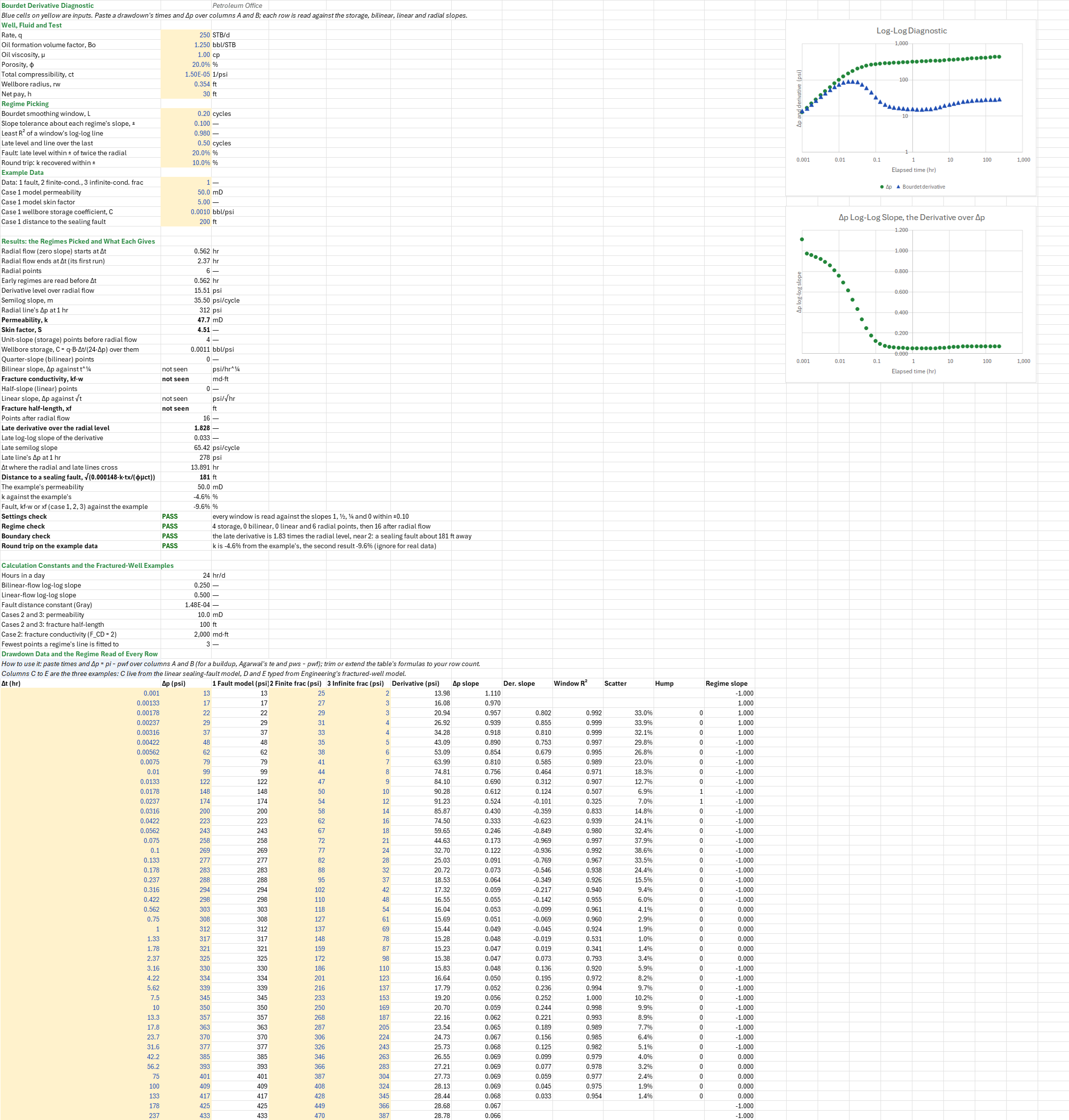
Description
Which flow regimes does a drawdown show, and what does each one give? You paste the times and the pressure drop and set the rate and the fluid and rock. Every row's derivative slope is read against the classic regimes: 1 for wellbore storage, ¼ for bilinear flow in a finite-conductivity fracture, ½ for linear flow and 0 for infinite-acting radial flow. You read off the storage coefficient C, the fracture conductivity kf·w, the half-length xf, and k and skin, each from its regime's straight line over its own points, and a boundary from the late derivative.
Parameters:
- Well and fluid: the rate and the fluid and rock (
BD_q,BD_Bo,BD_mu,BD_phi,BD_ct,BD_rw,BD_h) - Regime picking: the Bourdet smoothing window (
BD_L, 0.2), the slope tolerance about each regime's slope (BD_Tol, ±0.1), the least R² of a window's log-log line (BD_R2, 0.98), the late window (BD_Span, the last half log cycle), how close to twice the radial level a fault must be (BD_RTol, ±20 %), and the round-trip tolerance on k (BD_KTol, ±10 %) - Example data: which of three data sets fills the Δp column (
BD_Case), and the first one's model: k, skin, C and the fault distance (BD_ModelK,BD_ModelS,BD_C,BD_Lb) - Data: Δt and Δp, the region
BD_Data
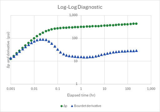
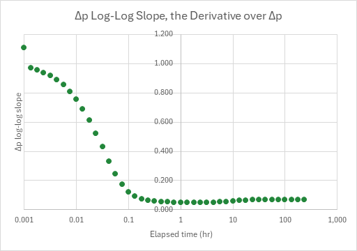
How to use it: Paste the times and Δp = pi − pwf over columns A and B, and set the rate and the fluid and rock. For a buildup, paste Agarwal's equivalent time te and pws − pwf. Keep the table's rows or trim its formulas to your row count. The example columns C to E and the round-trip check then don't apply. A log-log plot draws Δp and its derivative. A second plot draws Δp's own log-log slope, the derivative over Δp, against time: 1 in storage, ½ in linear and ¼ in bilinear flow, and falling in radial flow.
Method: The derivative is Bourdet's dΔp/d ln t, with smoothing window L. Each row gets two slopes. Δp's own log-log slope is the derivative over Δp. The derivative's slope is the least-squares slope of ln(derivative) against ln t over the five rows centred on it (SLOPE, RSQ). A row is read as one of the regime slopes, written in the Regime slope column:
- Radial flow (0) when the derivative's slope is within ±Tol of 0, its R² is at least the least R² set or its five values scatter less than Tol/2 about their mean (a flat line has no R²), and the middle three don't stand above both ends by more than Tol/2 (that is the storage hump's top).
- Linear (½) or bilinear (¼) when both slopes are within ±Tol of ½ or ¼ and R² is at least the least R² set.
- Storage (1) when Δp's slope is within ±Tol of 1; any other row is −1.
Asking Δp's slope to agree as well is what keeps out the slopes the derivative only passes through. The storage hump's rising side crosses ½, and the step up to a fault's doubled level crosses ¼, but Δp's slope is near 0.8 and 0.05 there. Radial flow is the first unbroken run of radial rows. Storage, bilinear and linear points count only before it starts, and every row after it is the boundary's.
- Regime lines. Each regime's line is fitted over its rows only, by
FILTER. C = q·B·Δt/(24·Δp), averaged over the storage points. The bilinear line is Δp against t^¼, so kf·w = [44.1·q·B·μ/(h·m)]²/√(φμct·k) (the bilinear-flow fit). The linear line is Δp against √t, so xf·√k = 4.064·q·B/(m·h)·√(μ/(φct)) (the square-root-of-time fit). The MDH line is Δp against log₁₀ t, so k = 162.6·q·B·μ/(m·h) and S = 1.151·[Δp1hr/m − log₁₀(k/(φμct·rw²)) + 3.23] (the MDH fit). The fracture fits take that k. - Boundary. After radial flow, the late derivative's level and slope tell a boundary: twice the radial level is a sealing fault. Over the last half log cycle (the late window), the sheet reads the derivative's mean over the radial level and its log-log slope. It also fits a second semilog line, and where it crosses the MDH line at tx, a fault lies at √(0.000148·k·tx/(φμct)) (Gray).
Example: The well and fluid are the PTA reference well the buildup sheets share: 250 STB/d, Bo 1.25 bbl/STB, μ 1 cp, φ 20 %, ct 1.5 × 10⁻⁵ 1/psi, rw 0.354 ft and h 30 ft. Case 1, the default, is the Buildup Boundary Signatures sheet's well (k 50 mD, S 5, C 0.001 bbl/psi) 200 ft from a sealing fault, drawn down from 0.001 to 237 hr by the add-in's linear sealing-fault model. Four points from 0.00133 hr sit at unit slope and give C = 0.00107 bbl/psi. Radial flow runs from 0.562 to 2.37 hr, 6 points at a derivative of 15.51 psi. The MDH line gives m = 35.50 psi/cycle, so k = 47.72 mD and S = 4.51, 4.6 % and 0.49 below the model's, within ±10 %. The 16 points after it climb to 1.83 times the radial level, a sealing fault. The late line has m = 65.42 psi/cycle and crosses the MDH line at 13.9 hr, which puts the fault 181 ft away, 9.6 % short of the model's 200 ft. The Buildup Boundary Signatures sheet reads the same fault at 1.83 and 180 ft from its buildup. No bilinear or linear points are found.
Cases 2 and 3 are a hydraulically fractured well in the same well and fluid but 10 mD rock: a 100 ft fracture of finite conductivity (FCD = 2, kf·w = 2,000 md·ft) and of infinite conductivity. No PO function models a fractured well, so their Δp are typed from the Engineering library's fractured vertical-well model (no storage, no skin). In case 2, 23 points from 0.0133 to 7.5 hr are bilinear, with a slope of 140.9 psi/hr^¼. Radial flow from 17.8 to 133 hr gives k = 10.48 mD and S = −4.25, so kf·w = 1,895 md·ft, 5.2 % short of the model's. In case 3, 17 points from 0.00178 to 0.178 hr are linear, with a slope of 76.54 psi/√hr. Radial flow from 23.7 hr gives k = 10.48 mD and S = −4.84, so xf = 98.6 ft against the model's 100. Both skins are the fracture's: Cinco-Ley's equivalent radius gives −4.37 at FCD = 2, and Prats' xf/2 gives −4.95. The fits read 0.1 lower because the derivative is still 5 % under its level when the run starts, which also puts k 4.8 % high.
The sheet was checked against a standalone script that rebuilds the three data sets from the Engineering library's models (the vertical-well model with a linear sealing fault, and the fractured vertical-well model). It takes the library's Bourdet derivative, which equals the sheet's at every interior point, and applies the sheet's regime rule. For the lines it uses its own least squares with the library's buildup permeability-from-slope, Horner skin and fault distance from the intersection time. It reproduces every number above to 10⁻⁸. The library's own regime finders (a five-point window at ±0.1 and R² 0.98) return the same storage, radial and bilinear windows. They report each one two points wider at each end, the window's half-width, and drop the end points, where the library's derivative isn't defined. They also show what the Δp-slope test removes: a "linear" stretch on the storage hump and a "bilinear" one on the step to the fault in case 1. No printed example interprets a full derivative by regime with every input given, so the sheet is not compared with a published one.
Functions used
PO.PTA.Pw.VW.LinSealF(time, prod_data, B, Ul, C, Rw, S, Ct, porosity, h, K, L)
Calculates wellbore pressure drop for vertical well in infinite homogeneous reservoir with linear sealing fault boundary, [psi].
PO.DCA.Diag.Bourdet.SemiLog(x_values, y_values, t, L)
Calculates the classical Bourdet derivative dy/d(ln x) at point t, the log-domain estimator used for semilog and log-log well-test analysis. Multiply by LN(10) for a slope per log cycle.
Names (69)
| Name | Refers to | Comment |
|---|---|---|
PO.PTA.MDH.FitLAMBDA |
=LAMBDA(t, dp, q, B, mu, h, phi, ct, rw, output, LET(x, LOG10(t), m, SLOPE(dp, x), dp_1h, INTERCEPT(dp, x), perm, 162.6*q*B*mu/(m*h), skin, 1.151*(dp_1h/m-LOG10(perm/(phi*mu*ct*rw^2))+3.23), IF(m<=0, NA(), IF(output="k", perm, IF(output="S", skin, IF(output="m", m, IF(output="dp1h", dp_1h, NA()))))))) |
MDH semilog straight-line fit of a drawdown: least squares of Δp against log10(t) over the points given; output "k" [mD], "S" [dimensionless], "m" [psi/cycle] or "dp1h" [psi], the line's Δp at 1 h. |
PO.PTA.Bilinear.FitLAMBDA |
=LAMBDA(t, dp, q, B, mu, h, phi, ct, k, output, LET(x, t^0.25, m, SLOPE(dp, x), icpt, INTERCEPT(dp, x), kfw, (141.2*2.4508334*0.0002637^0.25*q*B*mu/(h*m))^2/SQRT(phi*mu*ct*k), IF(m<=0, NA(), IF(output="m", m, IF(output="b", icpt, IF(output="kfw", kfw, NA())))))) |
Bilinear-flow fit of a fractured well: least squares of Δp against Δt^¼ (h) over the points given; output "m" [psi/h^¼], "b" [psi] or "kfw" [md·ft], the fracture conductivity from the slope. |
PO.PTA.Linear.SqrtTLAMBDA |
=LAMBDA(t, dp, q, B, mu, h, phi, ct, k, output, LET(x, SQRT(t), m, SLOPE(dp, x), icpt, INTERCEPT(dp, x), xfrk, 141.2*SQRT(PI()*0.0002637)*q*B/(m*h)*SQRT(mu/(phi*ct)), IF(m<=0, NA(), IF(output="m", m, IF(output="b", icpt, IF(output="xfrk", xfrk, IF(output="xf", xfrk/SQRT(k), NA()))))))) |
Linear-flow fit of a fractured well: least squares of Δp against √Δt (h) over the points given; output "m" [psi/√h], "b" [psi], "xfrk" [ft·md^½] or "xf" [ft] at the permeability given. |
BD_q |
$B$4 |
Rate, q, STB/d |
BD_Bo |
$B$5 |
Oil formation volume factor, Bo, bbl/STB |
BD_mu |
$B$6 |
Oil viscosity, μ, cp |
BD_phi |
$B$7 |
Porosity, φ, % |
BD_ct |
$B$8 |
Total compressibility, ct, 1/psi |
BD_rw |
$B$9 |
Wellbore radius, rw, ft |
BD_h |
$B$10 |
Net pay, h, ft |
BD_L |
$B$12 |
Bourdet smoothing window, L, cycles |
BD_Tol |
$B$13 |
Slope tolerance about each regime's slope, ± |
BD_R2 |
$B$14 |
Least R² of a window's log-log line |
BD_Span |
$B$15 |
Late level and line over the last, cycles |
BD_RTol |
$B$16 |
Fault: late level within ± of twice the radial, % |
BD_KTol |
$B$17 |
Round trip: k recovered within ±, % |
BD_Case |
$B$19 |
Data: 1 fault, 2 finite-cond., 3 infinite-cond. frac |
BD_ModelK |
$B$20 |
Case 1 model permeability, mD |
BD_ModelS |
$B$21 |
Case 1 model skin factor |
BD_C |
$B$22 |
Case 1 wellbore storage coefficient, C, bbl/psi |
BD_Lb |
$B$23 |
Case 1 distance to the sealing fault, ft |
BD_Inputs |
$B$4:$B$23 |
Rate, fluid and rock, the Bourdet window, the slope tolerance and R², the late window, the fault and round-trip limits, and which example the data is |
BD_RadStart |
$B$26 |
Radial flow (zero slope) starts at Δt, hr |
BD_RadEnd |
$B$27 |
Radial flow ends at Δt (its first run), hr |
BD_NRad |
$B$28 |
Radial points |
BD_Before |
$B$29 |
Early regimes are read before Δt, hr |
BD_Level |
$B$30 |
Derivative level over radial flow, psi |
BD_M |
$B$31 |
Semilog slope, m, psi/cycle |
BD_Dp1h |
$B$32 |
Radial line's Δp at 1 hr, psi |
BD_K |
$B$33 |
Permeability, k, mD |
BD_S |
$B$34 |
Skin factor, S |
BD_NSto |
$B$35 |
Unit-slope (storage) points before radial flow |
BD_Cfit |
$B$36 |
Wellbore storage, C = q·B·Δt/(24·Δp) over them, bbl/psi |
BD_NBil |
$B$37 |
Quarter-slope (bilinear) points |
BD_mBil |
$B$38 |
Bilinear slope, Δp against t^¼, psi/hr^¼ |
BD_Kfw |
$B$39 |
Fracture conductivity, kf·w, md·ft |
BD_NLin |
$B$40 |
Half-slope (linear) points |
BD_mLin |
$B$41 |
Linear slope, Δp against √t, psi/√hr |
BD_Xf |
$B$42 |
Fracture half-length, xf, ft |
BD_NBnd |
$B$43 |
Points after radial flow |
BD_Ratio |
$B$44 |
Late derivative over the radial level |
BD_LateSlope |
$B$45 |
Late log-log slope of the derivative |
BD_mLate |
$B$46 |
Late semilog slope, psi/cycle |
BD_bLate |
$B$47 |
Late line's Δp at 1 hr, psi |
BD_Tx |
$B$48 |
Δt where the radial and late lines cross, hr |
BD_Dist |
$B$49 |
Distance to a sealing fault, √(0.000148·k·tx/(φμct)), ft |
BD_KModel |
$B$50 |
The example's permeability, mD |
BD_KErr |
$B$51 |
k against the example's, % |
BD_XErr |
$B$52 |
Fault, kf·w or xf (case 1, 2, 3) against the example, % |
BD_SetCheck |
$B$53 |
Settings check verdict |
BD_SetCheckNote |
$C$53 |
Settings check comment |
BD_RegimeCheck |
$B$54 |
Regime check verdict |
BD_RegimeCheckNote |
$C$54 |
Regime check comment |
BD_BoundaryCheck |
$B$55 |
Boundary check verdict |
BD_BoundaryCheckNote |
$C$55 |
Boundary check comment |
BD_TripCheck |
$B$56 |
Round trip on the example data verdict |
BD_TripCheckNote |
$C$56 |
Round trip on the example data comment |
BD_Results |
$B$26:$B$56 |
Each regime's points and fit: C, kf·w, xf, the radial window, k and S, the late level and slope, the fault distance, the round trip and the checks |
BD_Hr |
$B$59 |
Hours in a day, hr/d |
BD_SBil |
$B$60 |
Bilinear-flow log-log slope |
BD_SLin |
$B$61 |
Linear-flow log-log slope |
BD_Gray |
$B$62 |
Fault distance constant (Gray) |
BD_FracK |
$B$63 |
Cases 2 and 3: permeability, mD |
BD_FracXf |
$B$64 |
Cases 2 and 3: fracture half-length, ft |
BD_MinN |
$B$66 |
Fewest points a regime's line is fitted to |
BD_FracKfw |
$B$65 |
Case 2: fracture conductivity (F_CD = 2), md·ft |
BD_Data |
$A$71:$E$114 |
Elapsed time and Δp (the chosen example's until you paste a gauge's), and the three examples |
BD_Analysis |
$F$71:$L$114 |
Per row: the Bourdet derivative, Δp's log-log slope, the derivative's slope, R², scatter and hump over five rows, and the regime, as its slope: 1 storage, ¼ bilinear, ½ linear, 0 radial, −1 none |
BD_Curve |
$A$71:$F$114 |
Log-Log Diagnostic |
Details
| Inserts | 114 rows × 12 columns |
| Category | Pressure Transient Analysis |
| For agents and tools | Descriptor (.md) |