DFIT G-Function Analysis
Description
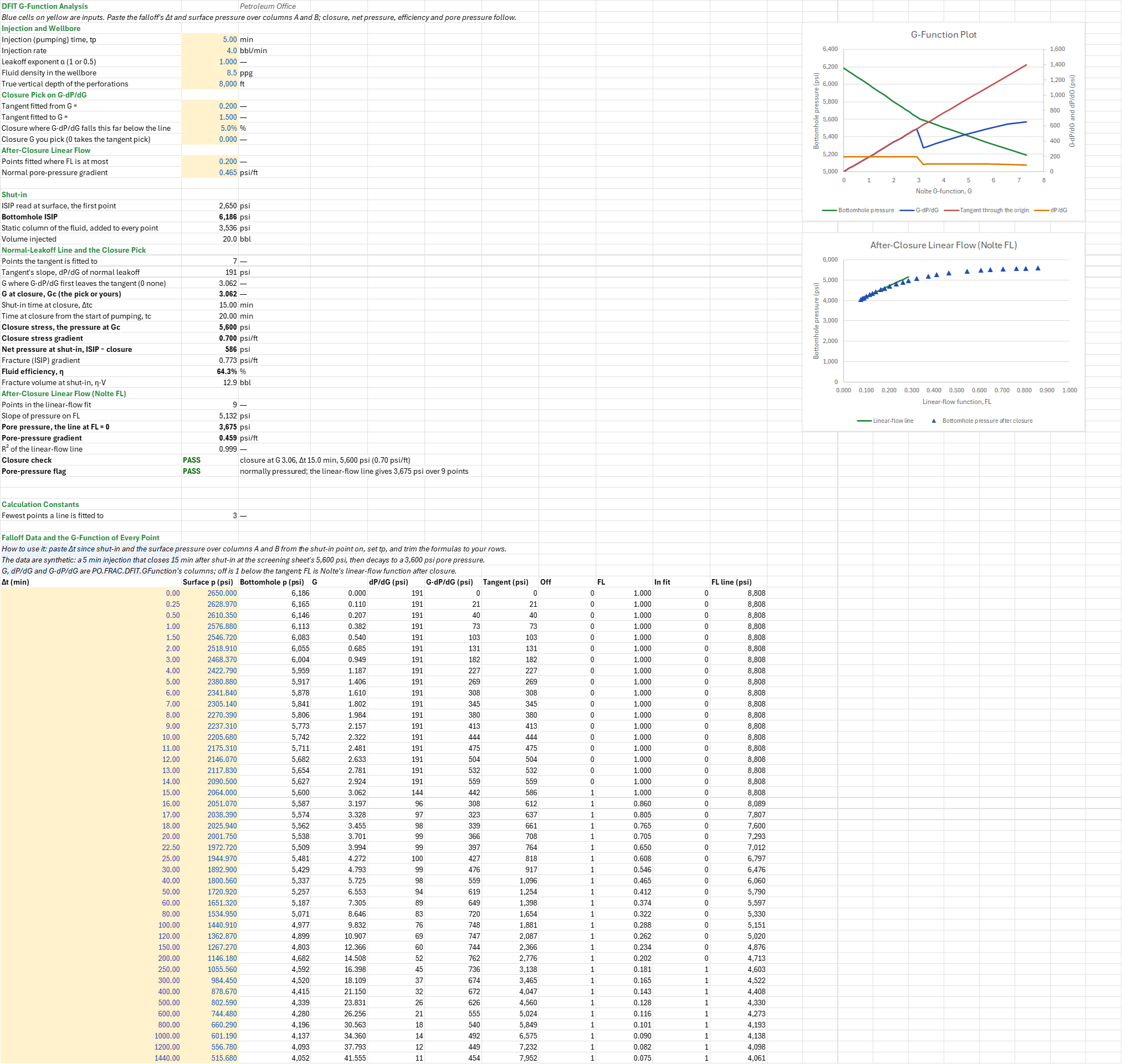
Where did the minifrac's fracture close and at what stress, how much net pressure held it open, how efficient was the fluid, and what is the pore pressure? You enter a diagnostic fracture injection test (DFIT): the injection time and rate, the fluid and depth, and the falloff's shut-in times and surface pressures. You read off the bottomhole ISIP, the closure picked on Nolte's G-function, the closure stress, the net pressure, the fluid efficiency and the fracture volume at shut-in, and the pore pressure from the after-closure line.
Parameters:
- Injection and wellbore: the injection time
DFIT_Tp, the rateDFIT_Q, the leakoff exponentDFIT_Alpha(1 or 0.5), the fluid density in the holeDFIT_RhoFluidand the depthDFIT_Tvd - Closure pick: the G window the tangent is fitted over (
DFIT_GLo,DFIT_GHi), how far below it a point must fall to be closureDFIT_Tol, and your own closure GDFIT_GcUser(0 takes the pick) - After closure: the largest FL fitted
DFIT_FLMaxand the normal pore-pressure gradientDFIT_NormalGrad - Data: Δt since shut-in and the surface pressure, the region
DFIT_Data
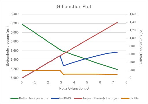
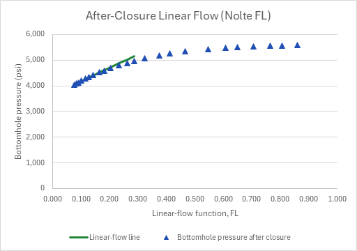
How to use it: Read the test the way a frac engineer does before the main treatment. Paste Δt since shut-in and the surface pressure over columns A and B, starting with the shut-in point, set tp and the rate, and trim the formulas to your rows. A downhole gauge's record goes in column B with the fluid density set to 0, so the column adds nothing. Smooth a noisy record before the derivative is read, set the tangent window past any early tortuosity or storage, and check the pick by eye on the G-function plot; your own closure G overrides the pick. The sheet adds the static column to the surface pressure, computes G, dP/dG and the superposition derivative G·dP/dG one element a cell, and picks closure by tangent deviation: a straight line through the origin is fitted to G·dP/dG over a window of early G, and closure is the first point that falls a set fraction below it. The pick is yours to override. After closure, a least-squares line of pressure against Nolte's linear-flow function FL gives the pore pressure at FL = 0, flagged against a normal gradient. A G-function plot and an after-closure plot draw both reads. The synthetic falloff is a stand-in for data.
Method: The bottomhole pressure is the surface pressure plus the static column, so the bottomhole ISIP is the surface ISIP + 0.052·ρ·TVD. With ΔtD = Δt/tp, Nolte's g = (4/3)·[(1 + ΔtD)^1.5 − ΔtD^1.5] for α = 1 and G = (4/π)·(g − 4/3); dP/dG is a central difference and G·dP/dG its product with G. While the fracture is open with normal leakoff the pressure falls on a straight line in G, so G·dP/dG lies on a line through the origin; its slope is the least-squares fit Σ G·(G·dP/dG)/Σ G² over the G window. Closure is the first point past the window's start whose G·dP/dG is more than the set fraction below that line. The closure time and stress at Gc are interpolated linearly in G between the points either side. The net pressure is the bottomhole ISIP − pc, and the fluid efficiency is η = Gc/(Gc + 4·g0/π), Gc/(Gc + 1.698) for α = 1; η times the volume injected is the fracture volume at shut-in. After closure, FL = (2/π)·asin(√(tc/t)), with t from the start of pumping and tc = tp + Δtc (Nolte 1997). In reservoir linear flow p = pr + mL·FL, so the least-squares line through the after-closure points with FL up to the largest FL fitted gives pr at FL = 0.
Example: The default is a minifrac ahead of the Fracture Design Screening (Unified Fracture Design) treatment, at the same 8,000 ft with 8.5 ppg fluid in the hole: 20 bbl pumped at 4 bbl/min for 5 min, shut in at 2,650 psi at surface, and read for a day. The falloff is synthetic. It falls on the normal-leakoff line from the screening sheet's 6,186 psi bottomhole ISIP to its 5,600 psi closure, 15 min after shut-in, and then decays towards a 3,600 psi (0.45 psi/ft) pore pressure, its first post-closure decline half the pre-closure rate.
The 3,536 psi column puts the ISIP at 6,186 psi at the perforations. Seven points from G = 0.21 to 1.41 fit a tangent of slope 191.36 psi, and the first point to fall more than 5 % below it is at Δt = 15 min, G = 3.062: G·dP/dG is 442 there against the line's 586, because its central difference already takes in the slower decline after closure. Closure is at 5,600 psi, 0.700 psi/ft, and the net pressure at shut-in is 586 psi, the screening sheet's. The efficiency is 3.062/(3.062 + 1.698) = 64.3 %, so 12.9 of the 20 bbl were still in the fracture at shut-in. Nine after-closure points have FL ≤ 0.2 (Δt from 250 min). Their line has a slope of 5,132 psi and an R² of 0.9985, and meets FL = 0 at 3,675 psi, 0.459 psi/ft: normally pressured, under the 0.465 psi/ft normal gradient. The intercept reads 75 psi (2 %) above the model's 3,600 psi, because a day's falloff hasn't reached pure linear flow; FL ≤ 0.1 (three points) reads 3,625 psi.
Functions used
None: the blueprint calculates with Excel's own functions.
Names (45)
| Name | Refers to | Comment |
|---|---|---|
PO.FRAC.Eval.ISIPLAMBDA |
=LAMBDA(isip_surf, rho_fluid, tvd, closure, output, IF(OR(rho_fluid<0, tvd<=0), NA(), LET(isip_bh, isip_surf+0.052*rho_fluid*tvd, IF(output="ISIP", isip_bh, IF(output="Pnet", isip_bh-closure, IF(output="Gradient", isip_bh/tvd, NA())))))) |
Instantaneous shut-in pressure at the fracture from the surface ISIP plus the static column 0.052·ρ·TVD; output "ISIP" (psi), "Pnet" (ISIP − closure, psi) or "Gradient" (psi/ft). |
PO.FRAC.DFIT.GFunctionLAMBDA |
=LAMBDA(dt, tp, p, alpha, output, IF(OR(tp<=0, AND(alpha<>1, alpha<>0.5)), NA(), LET(td, dt/tp, gn, IF(alpha=1, 4/3*((1+td)^1.5-td^1.5), (1+td)*ASIN(1/SQRT(1+td))+SQRT(td)), gz, IF(alpha=1, 4/3, PI()/2), bigg, 4/PI()*(gn-gz), cnt, ROWS(p), ix, SEQUENCE(cnt), jx, TRANSPOSE(ix), nxt, --(jx=ix+(ix<cnt)), prv, --(jx=ix-(ix>1)), dpdg, -(MMULT(nxt, p)-MMULT(prv, p))/(MMULT(nxt, bigg)-MMULT(prv, bigg)), sel, IF(output="dtD", 1, IF(output="gNolte", 2, IF(output="G", 3, IF(output="dPdG", 4, IF(output="GdPdG", 5, 0))))), IF(sel=0, NA(), CHOOSE(sel, td, gn, bigg, dpdg, bigg*dpdg))))) |
Nolte G-function of a fracture falloff for leakoff exponent alpha 1 or 0.5; output column "dtD", "gNolte" g(ΔtD), "G", "dPdG" (−dp/dG) or "GdPdG" (G·dP/dG), central differences. |
PO.FRAC.DFIT.EfficiencyLAMBDA |
=LAMBDA(Gc, alpha, IF(AND(alpha<>1, alpha<>0.5), NA(), IF(Gc<0, NA(), Gc/(Gc+4/PI()*IF(alpha=1, 4/3, PI()/2))))) |
Fracturing fluid efficiency from the G-function at closure (Nolte material balance): η = Gc/(Gc + 4·g0/π), Gc/(2 + Gc) for alpha 0.5 and Gc/(Gc + 16/(3π)) for alpha 1. |
DFIT_Tp |
$B$4 |
Injection (pumping) time, tp, min |
DFIT_Q |
$B$5 |
Injection rate, bbl/min |
DFIT_Alpha |
$B$6 |
Leakoff exponent α (1 or 0.5) |
DFIT_RhoFluid |
$B$7 |
Fluid density in the wellbore, ppg |
DFIT_Tvd |
$B$8 |
True vertical depth of the perforations, ft |
DFIT_GLo |
$B$10 |
Tangent fitted from G = |
DFIT_GHi |
$B$11 |
Tangent fitted to G = |
DFIT_Tol |
$B$12 |
Closure where G·dP/dG falls this far below the line, % |
DFIT_GcUser |
$B$13 |
Closure G you pick (0 takes the tangent pick) |
DFIT_FLMax |
$B$15 |
Points fitted where FL is at most |
DFIT_NormalGrad |
$B$16 |
Normal pore-pressure gradient, psi/ft |
DFIT_Inputs |
$B$4:$B$16 |
The injection, the fluid column and depth, the window and tolerance of the closure pick with its override, and the after-closure window |
DFIT_IsipSurf |
$B$19 |
ISIP read at surface, the first point, psi |
DFIT_Isip |
$B$20 |
Bottomhole ISIP, psi |
DFIT_Hydro |
$B$21 |
Static column of the fluid, added to every point, psi |
DFIT_Vinj |
$B$22 |
Volume injected, bbl |
DFIT_NFit |
$B$24 |
Points the tangent is fitted to |
DFIT_M |
$B$25 |
Tangent's slope, dP/dG of normal leakoff, psi |
DFIT_GcPick |
$B$26 |
G where G·dP/dG first leaves the tangent (0 none) |
DFIT_Gc |
$B$27 |
G at closure, Gc (the pick or yours) |
DFIT_DtC |
$B$28 |
Shut-in time at closure, Δtc, min |
DFIT_TcTotal |
$B$29 |
Time at closure from the start of pumping, tc, min |
DFIT_Pc |
$B$30 |
Closure stress, the pressure at Gc, psi |
DFIT_PcGrad |
$B$31 |
Closure stress gradient, psi/ft |
DFIT_Pnet |
$B$32 |
Net pressure at shut-in, ISIP − closure, psi |
DFIT_IsipGrad |
$B$33 |
Fracture (ISIP) gradient, psi/ft |
DFIT_Eta |
$B$34 |
Fluid efficiency, η, % |
DFIT_Vfrac |
$B$35 |
Fracture volume at shut-in, η·V, bbl |
DFIT_NAca |
$B$37 |
Points in the linear-flow fit |
DFIT_MAca |
$B$38 |
Slope of pressure on FL, psi |
DFIT_Pr |
$B$39 |
Pore pressure, the line at FL = 0, psi |
DFIT_PrGrad |
$B$40 |
Pore-pressure gradient, psi/ft |
DFIT_R2 |
$B$41 |
R² of the linear-flow line |
DFIT_ClosureCheck |
$B$42 |
Closure check verdict |
DFIT_ClosureCheckNote |
$C$42 |
Closure check comment |
DFIT_PoreCheck |
$B$43 |
Pore-pressure flag verdict |
DFIT_PoreCheckNote |
$C$43 |
Pore-pressure flag comment |
DFIT_Results |
$B$19:$B$43 |
The ISIP, the tangent and the closure pick, closure stress, net pressure and efficiency, the after-closure pore pressure, and the two checks |
DFIT_MinN |
$B$47 |
Fewest points a line is fitted to |
DFIT_Data |
$A$54:$B$96 |
The falloff: Δt since shut-in and the surface pressure, synthetic until you paste a gauge's |
DFIT_Analysis |
$C$54:$K$96 |
Per point: the bottomhole pressure, G, dP/dG and G·dP/dG, the tangent, the off-tangent flag, FL, the linear-flow window and its line |
DFIT_GPlot |
$C$54:$G$82 |
G-Function Plot |
Details
| Inserts | 96 rows × 11 columns |
| Category | Hydraulic Fracturing |
| For agents and tools | Descriptor (.md) |