Water-Oil Ratio Diagnostics
Description
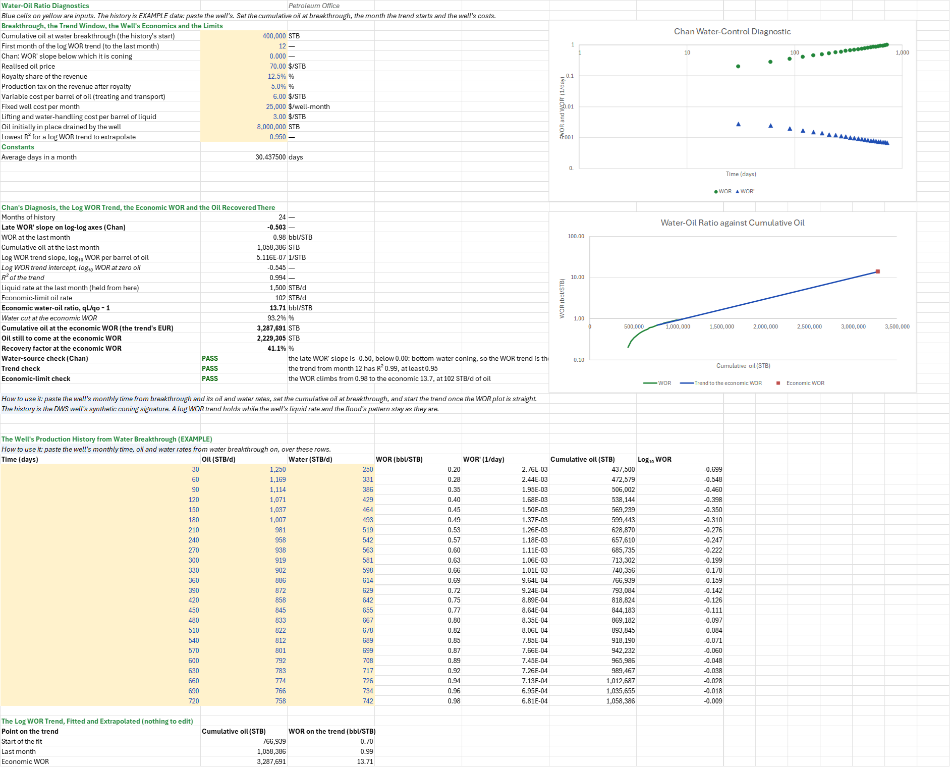
Where is a producer's water coming from, and how much more oil will the well make before the water makes it uneconomic? You enter the well's monthly oil and water rates from water breakthrough, its price, royalty, tax and costs, and the oil in place it drains. You read off on Chan's plot whether the water is coning or channelling, the economic WOR, and where the log WOR trend meets it: the well's EUR, the oil still to come and the recovery factor.
Parameters:
- History: the well's monthly time from breakthrough (days) and its oil and water rates (STB/d), in the history table
- Start: the cumulative oil at water breakthrough,
WOR_Np0(STB), and the first month of the trend's fit,WOR_FitFrom - Chan: the WOR′ slope below which the water reads as coning,
WOR_SlopeConing(0) - Economics: the oil price
WOR_Price($/STB), the royaltyWOR_Royaltyand production taxWOR_Tax, the variable cost per barrel of oilWOR_Opex, the fixed well cost per monthWOR_Fixed, and the lifting and water-handling cost per barrel of liquidWOR_Lift - Recovery: the oil initially in place the well drains,
WOR_N(STB) - Limits: the lowest R² of a trend to extrapolate,
WOR_R2Min
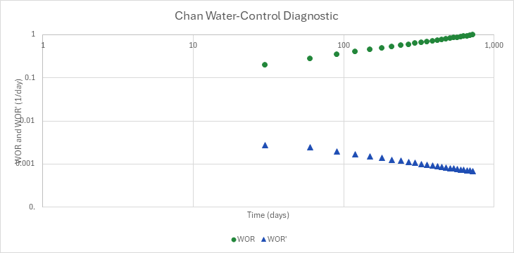
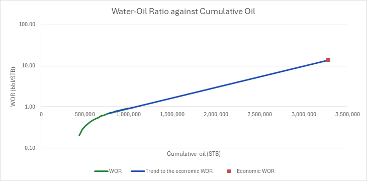
How to use it: The default history is a synthetic well. Paste your well's monthly time from breakthrough and its oil and water rates over the history table's rows; smooth noisy rates first. Set the cumulative oil at breakthrough from the well's production, the fit's first month where the log WOR plot turns straight, the costs from the lease operating statement, and the oil in place from a volumetric estimate or a decline-based one. The first chart is Chan's plot: the WOR and its time derivative WOR′ on log-log axes, whose late slope says whether the water is coning or channelling. The second draws the WOR against cumulative oil on a logarithmic WOR axis, with the trend from the fit's first month to the economic WOR. The water-source check reads coning when the late WOR′ slope is below the coning threshold and warns of channelling otherwise. The trend check fails when log WOR does not rise with cumulative oil, and warns when the fit's R² is below the limit. The economic-limit check warns when the well is already past its economic WOR.
Method: WOR = qw/qo. Chan's WOR′ at an interior month is the three-point derivative, the neighbouring slopes each weighted by the other interval; at the ends it is the one-sided slope. The late slope on log-log axes runs from the history's middle month to its second-to-last: log₁₀(WOR′ₗ/WOR′ₘ)/log₁₀(tₗ/tₘ). A falling WOR′ (a negative slope) is coning; a rising one is channelling.
The cumulative oil is Np₀ plus each month's qo Δt. Over the months from the fit's first month to the last, log₁₀ WOR = a + b Np by least squares. The well's liquid rate is held at its last month's qL, so its lifting cost is fixed. The economic-limit oil rate, the rate at which the well's oil no longer pays for its liquid, is qo,ec = (Fixed + qL · 30.4375 · Lift)/(Price (1 − Royalty)(1 − Tax) − Opex)/30.4375, and the economic WOR is qL/qo,ec − 1. The trend meets it at Np,ec = (log₁₀ WORec − a)/b, and the recovery factor is Np,ec/N.
Example: The default history is the downhole-water-sink ESP sizing sheet's well: 24 months of 1,500 STB/d of liquid whose WOR climbs from 0.20 to 0.98 as 0.2·√(t/30), a coning signature. The well had made 400,000 STB by water breakthrough. Oil sells at $70/STB with a 12.5% royalty and a 5% production tax; treating and transport cost $6 per barrel of oil, the well $25,000 a month, and lifting and water handling $3 per barrel of liquid. The well drains 8 MMSTB, and the trend is fitted from month 12.
Chan's late WOR′ slope is −0.503, as on the downhole-water-sink sheet: WOR′ falls with time, the signature of bottom-water coning. Hand check: log₁₀(6.9485 × 10⁻⁴ / 9.6384 × 10⁻⁴)/log₁₀(690/360) = −0.1421/0.2826 = −0.503. By the last month the well has made 1,058,386 STB at a WOR of 0.98. From month 12 the log WOR trend rises 5.116 × 10⁻⁷ decades per barrel, with R² 0.994. The well's netback is $52.19 per barrel of oil, and its fixed cost with the liquid's handling $161,969 a month, so it stops paying at 102.0 STB/d of oil: an economic WOR of 13.7, a 93.2% water cut. The trend reaches it at 3.29 MMSTB, another 2.23 MMSTB, 41.1% of the 8 MMSTB the well drains. Fitted over all 24 months, R² falls to 0.893 and the trend check warns, and the EUR falls to 2.25 MMSTB; from month 18 it is 3.63 MMSTB. At $30 per barrel of liquid the well stops paying at 878 STB/d, a WOR of 0.71, already passed.
Functions used
None: the blueprint calculates with Excel's own functions.
Names (40)
| Name | Refers to | Comment |
|---|---|---|
PO.PE.Chan.WORDerivativeLAMBDA |
=LAMBDA(time, wor, at, LET(n, COUNT(time), k, MATCH(at, time, 0), k_lo, MAX(1, k-1), k_hi, MIN(n, k+1), t_k, INDEX(time, k), t_lo, INDEX(time, k_lo), t_hi, INDEX(time, k_hi), w_k, INDEX(wor, k), w_lo, INDEX(wor, k_lo), w_hi, INDEX(wor, k_hi), IF(k=1, (w_hi-w_k)/(t_hi-t_k), IF(k=n, (w_k-w_lo)/(t_k-t_lo), ((w_k-w_lo)/(t_k-t_lo)*(t_hi-t_k)+(w_hi-w_k)/(t_hi-t_k)*(t_k-t_lo))/(t_hi-t_lo))))) |
Chan (1995) WOR′: the time derivative of the water-oil ratio at one point of a production history, a three-point difference weighted by the neighbouring intervals, [1/time unit]. |
PO.RES.Reserves.EconLimitLAMBDA |
=LAMBDA(Price, Royalty, Tax, Opex, Fixed, LET(netback, Price*(1-Royalty)*(1-Tax)-Opex, IF(netback>0, Fixed/netback, NA()))) |
Economic-limit rate: fixed cost per period over the netback per unit after royalty, production tax and variable opex; #N/A if the netback is not positive |
WOR_Np0 |
$B$4 |
Cumulative oil at water breakthrough (the history's start), STB |
WOR_FitFrom |
$B$5 |
First month of the log WOR trend (to the last month) |
WOR_SlopeConing |
$B$6 |
Chan: WOR′ slope below which it is coning |
WOR_Price |
$B$7 |
Realised oil price, $/STB |
WOR_Royalty |
$B$8 |
Royalty share of the revenue, % |
WOR_Tax |
$B$9 |
Production tax on the revenue after royalty, % |
WOR_Opex |
$B$10 |
Variable cost per barrel of oil (treating and transport), $/STB |
WOR_Fixed |
$B$11 |
Fixed well cost per month, $/well-month |
WOR_Lift |
$B$12 |
Lifting and water-handling cost per barrel of liquid, $/STB |
WOR_N |
$B$13 |
Oil initially in place drained by the well, STB |
WOR_R2Min |
$B$14 |
Lowest R² for a log WOR trend to extrapolate |
WOR_Inputs |
$B$4:$B$14 |
The cumulative oil at breakthrough, the trend's first month, the Chan coning slope, the oil price, royalty, tax and costs, the oil in place and the fit limit |
WOR_DaysPerMonth |
$B$16 |
Average days in a month, days |
WOR_Months |
$B$22 |
Months of history |
WOR_ChanSlope |
$B$23 |
Late WOR′ slope on log-log axes (Chan) |
WOR_WorLast |
$B$24 |
WOR at the last month, bbl/STB |
WOR_NpLast |
$B$25 |
Cumulative oil at the last month, STB |
WOR_B |
$B$26 |
Log WOR trend slope, log₁₀ WOR per barrel of oil, 1/STB |
WOR_A |
$B$27 |
Log WOR trend intercept, log₁₀ WOR at zero oil |
WOR_R2 |
$B$28 |
R² of the trend |
WOR_QL |
$B$29 |
Liquid rate at the last month (held from here), STB/d |
WOR_QoEc |
$B$30 |
Economic-limit oil rate, STB/d |
WOR_WorEc |
$B$31 |
Economic water-oil ratio, qL/qo − 1, bbl/STB |
WOR_FwEc |
$B$32 |
Water cut at the economic WOR, % |
WOR_NpEc |
$B$33 |
Cumulative oil at the economic WOR (the trend's EUR), STB |
WOR_Rem |
$B$34 |
Oil still to come at the economic WOR, STB |
WOR_RF |
$B$35 |
Recovery factor at the economic WOR, % |
WOR_ChanCheck |
$B$36 |
Water-source check (Chan) verdict |
WOR_ChanCheckNote |
$C$36 |
Water-source check (Chan) comment |
WOR_TrendCheck |
$B$37 |
Trend check verdict |
WOR_TrendCheckNote |
$C$37 |
Trend check comment |
WOR_EconCheck |
$B$38 |
Economic-limit check verdict |
WOR_EconCheckNote |
$C$38 |
Economic-limit check comment |
WOR_Results |
$B$22:$B$38 |
The months, Chan's late slope, the last WOR and cumulative oil, the log WOR trend and its R², the economic oil rate and WOR, the oil recovered there and three checks |
WOR_History |
$A$47:$G$70 |
The well's monthly time, oil and water rates, its WOR and Chan's WOR′, the cumulative oil and log WOR |
WOR_Trend |
$A$74:$C$76 |
The fitted log WOR trend at the fit's start, at the last month and at the economic WOR |
WOR_ChanCurve |
$A$47:$E$70 |
Chan Water-Control Diagnostic |
WOR_TrendCurve |
$C$47:$F$70 |
Water-Oil Ratio against Cumulative Oil |
Details
| Inserts | 76 rows × 7 columns |
| Category | Decline Curve Analysis |
| For agents and tools | Descriptor (.md) |