Quick-Look Petrophysical Interpretation
Description
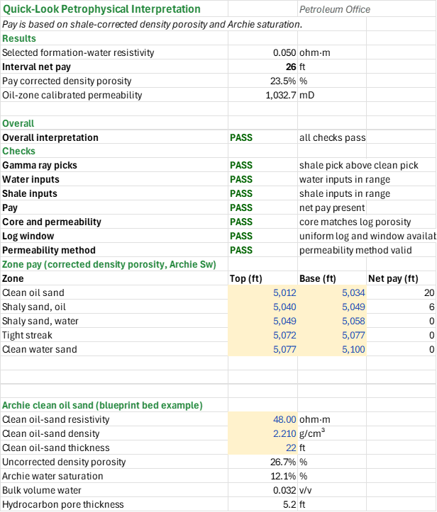
How much net pay does this log interval hold, at what porosity and saturation, and how permeable is it? You paste the interval's gamma ray, SP, density, neutron, sonic and deep resistivity and the core plugs, and pick the shale lines, water resistivity and cutoffs. You read off shale volume and porosity, water saturation by Archie and four shaly-sand models, gross, net reservoir and net pay per zone, and a core-calibrated permeability. Depth in ft, resistivity in ohm m, permeability in mD; porosity, saturation and Vsh as fractions.
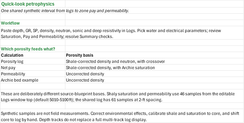
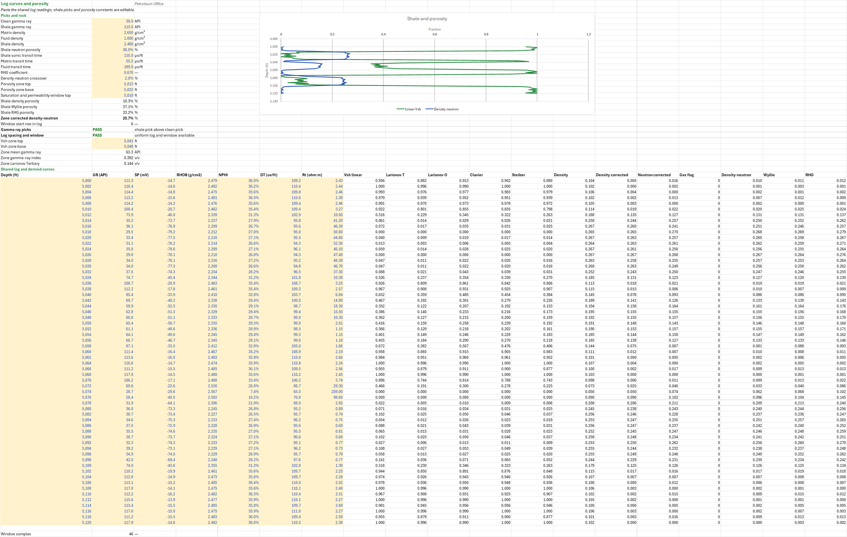
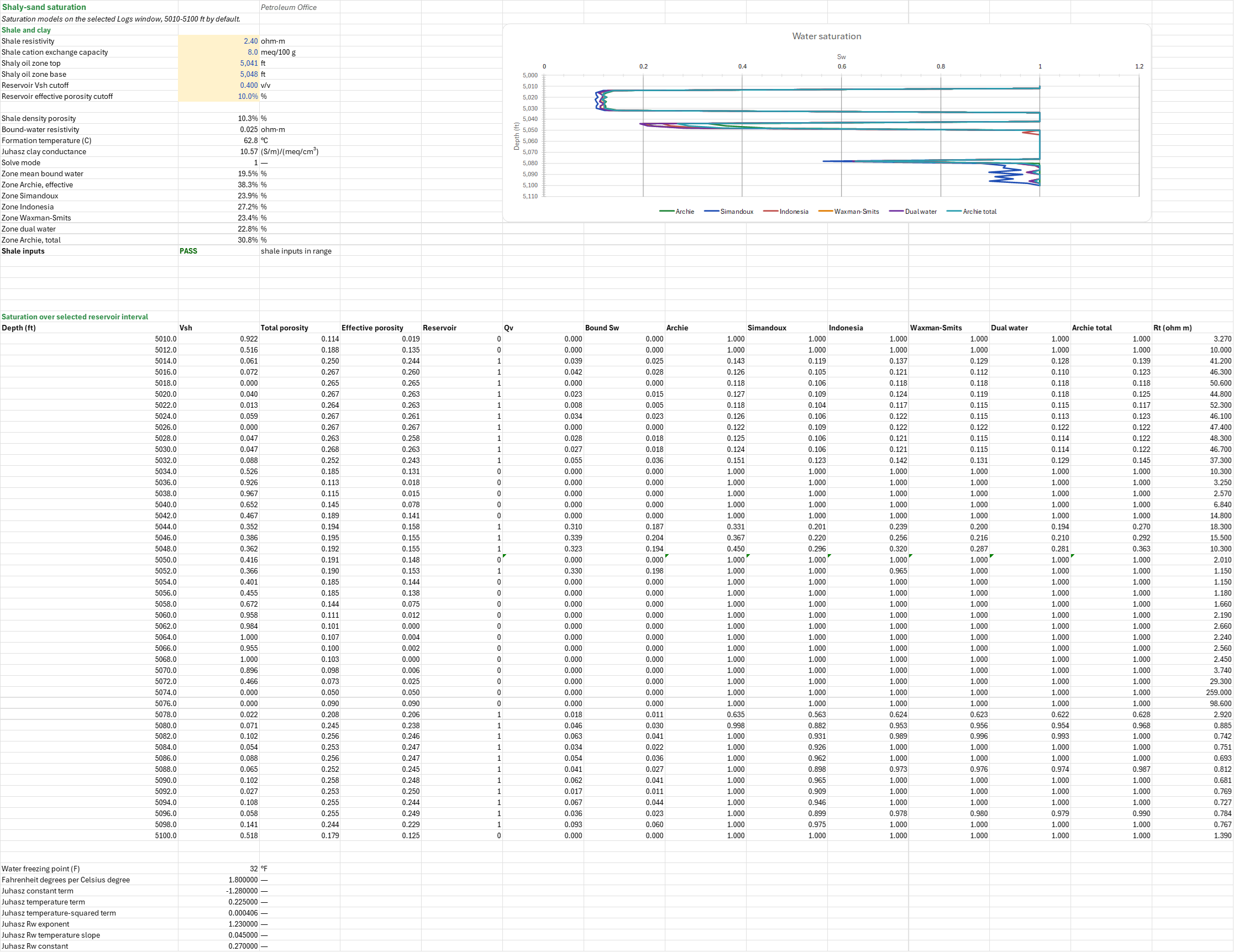
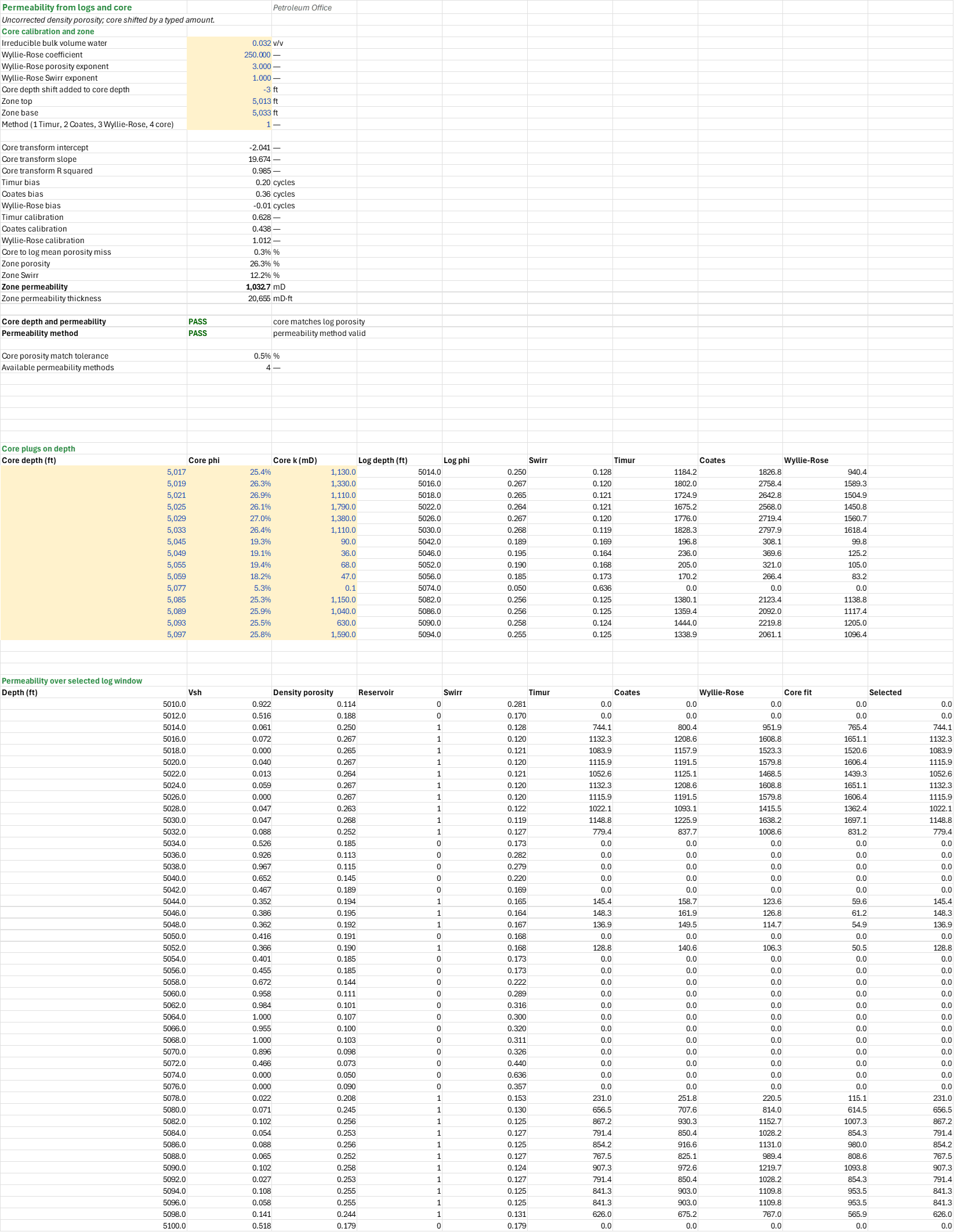
How to use it: Replace the blue log cells on the Logs sheet and the core cells on the Permeability sheet. The tables and formulas have fixed lengths: all 61 log depths must be numeric and increase uniformly by 2 ft, so resize the ranges and formulas before adding samples. Shaly saturation and permeability use a fixed 46-sample, 90-ft window at 2-ft spacing, starting at the editable window top on the Logs sheet (5010 ft by default); the selected window must lie inside the log, and the shifted core plugs inside the window. On the Water sheet compare the SP, minimum Rwa, Pickett and salinity estimates and select method 1-4 to link one, or keep the fixed Rw. Net pay uses the full interval but counts only the samples inside the typed gross window. Type the core-to-log depth shift by hand. Read the zone pay, Rw, porosity, permeability and every check on the Summary.
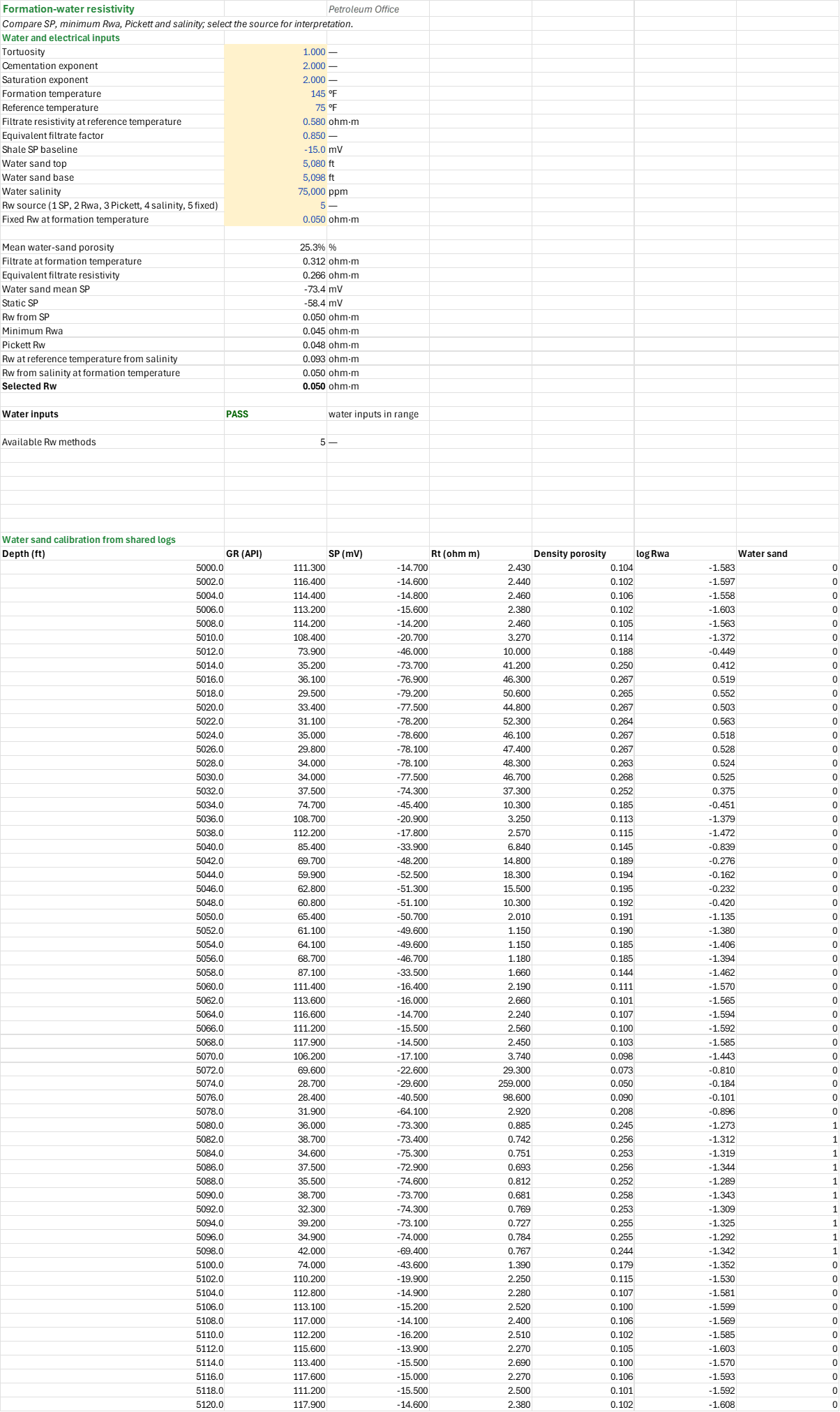
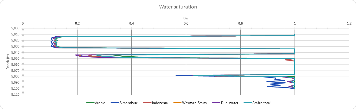
Method: Shale volume from the gamma-ray index and its Larionov (Tertiary and older rocks), Clavier and Steiber transforms; porosity from density, neutron-density and sonic (Wyllie and Raymer-Hunt-Gardner), each shale-corrected. Formation-water resistivity from four independent estimates: SP, minimum Rwa in the water sand, a Pickett plot and salinity, each brought to formation temperature. Water saturation by Archie, Sw = (a Rw/(phi^m Rt))^(1/n), and by Simandoux, Indonesia, Waxman-Smits and dual water. A sample is net reservoir when its Vsh and porosity pass their cutoffs, and net pay when its Archie Sw also passes. Permeability by Timur, Coates and Wyllie-Rose, each scaled to the core plugs, or by a core porosity-permeability fit. The computed curves and zone averages share the same log readings; the porosity bases differ, as set out under Validity.
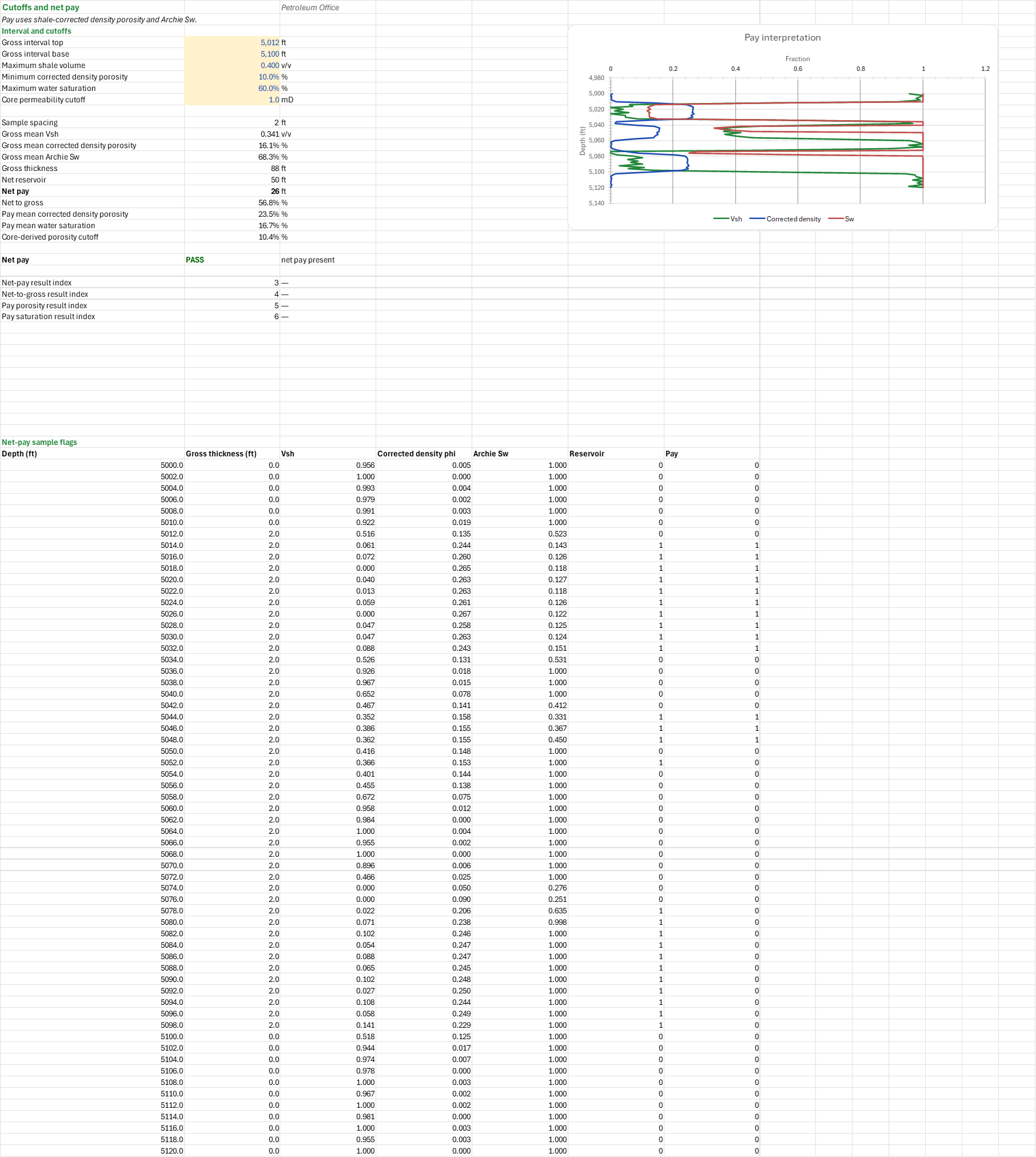
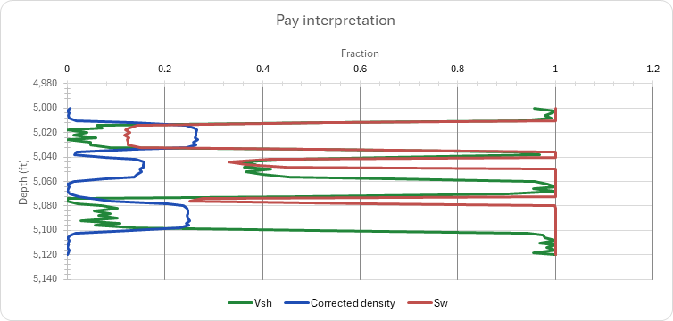
Example: The shared synthetic log interval from 5000 to 5120 ft in 2 ft samples, with 15 synthetic core plugs. With clean and shale gamma-ray picks of 30/115 API, Rw = 0.05 ohm m (the default fixed Rw, kept so the other source examples stay comparable) and cutoffs Vsh = 0.4, porosity = 0.10 and Sw = 0.60, the interval holds 88 ft gross, 50 ft net reservoir and 26 ft net pay. The calibrated Timur permeability of the clean oil zone is 1,032.725487 mD, and its corrected density-neutron porosity averages 0.257258396. These numbers match the source calculations on identical inputs and are synthetic, not field measurements.
Validity
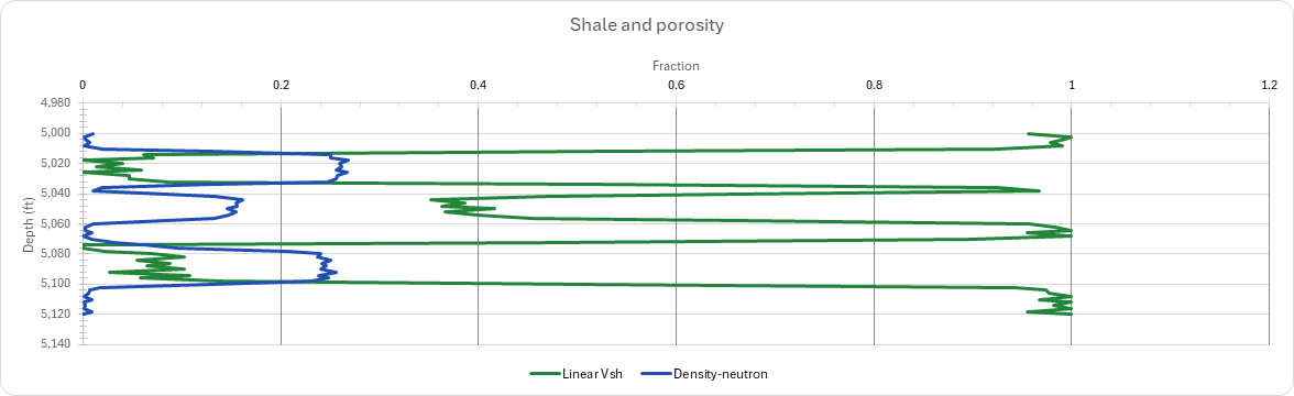
Net pay uses shale-corrected density porosity and Archie Sw, while the permeability model uses uncorrected density porosity. The porosity log's density-neutron curve combines separately shale-corrected density and neutron; the Archie bed example uses uncorrected density. Do not compare these as though they were one porosity measurement. Each zone's pay on the Summary uses the net-pay basis. The depth-track charts are simple XY depth tracks, not a full multi-track LAS viewer, and omit specialised log-track features. Correct logs for environmental effects and calibrate shale volume, saturation and permeability to the same rock and fluids. The example and core are synthetic.
The workbook does not match the core to the log automatically: the core-to-log shift is typed, not fitted. Permeability is an estimate, not a well test. Archie assumes a clean formation; calibrate the shaly-sand alternatives against core.
References
- Archie, G.E. (1942). The Electrical Resistivity Log as an Aid in Determining Some Reservoir Characteristics. Trans. AIME 146, 54-62.
- Wyllie, M.R.J. and Rose, W.D. (1950). Some Theoretical Considerations Related to the Quantitative Evaluation of the Physical Characteristics of Reservoir Rock from Electrical Log Data. Trans. AIME 189, 105-118.
- Wyllie, M.R.J., Gregory, A.R. and Gardner, L.W. (1956). Elastic Wave Velocities in Heterogeneous and Porous Media. Geophysics 21(1), 41-70.
- Pickett, G.R. (1966). A Review of Current Techniques for Determination of Water Saturation from Logs. JPT 18(11), 1425-1433.
- Timur, A. (1968). An Investigation of Permeability, Porosity, and Residual Water Saturation Relationships for Sandstone Reservoirs. The Log Analyst 9(4).
- Waxman, M.H. and Smits, L.J.M. (1968). Electrical Conductivities in Oil-Bearing Shaly Sands. SPE Journal 8(2), 107-122.
- Poupon, A. and Leveaux, J. (1971). Evaluation of Water Saturation in Shaly Formations. SPWLA 12th Annual Logging Symposium.
- Raymer, L.L., Hunt, E.R. and Gardner, J.S. (1980). An Improved Sonic Transit Time-to-Porosity Transform. SPWLA 21st Annual Logging Symposium.
- Clavier, C., Coates, G. and Dumanoir, J. (1984). Theoretical and Experimental Bases for the Dual-Water Model for Interpretation of Shaly Sands. SPE Journal 24(2), 153-168.
- Asquith, G. and Krygowski, D. (2004). Basic Well Log Analysis, 2nd ed. AAPG Methods in Exploration 16.
Inputs
| Input | Unit | Default | Name |
|---|---|---|---|
| Clean gamma ray | API | 30 | QLP_GRcl |
| Shale gamma ray | API | 115 | QLP_GRsh |
| Matrix density | g/cm3 | 2.65 | QLP_RhoMa |
| Fluid density | g/cm3 | 1 | QLP_RhoF |
| Saturation and permeability window top | ft | 5010 | QLP_WindowTop |
| Tortuosity | — | 1 | QLR_a |
| Cementation exponent | — | 2 | QLR_m |
| Saturation exponent | — | 2 | QLR_n |
| Rw source (1 SP, 2 Rwa, 3 Pickett, 4 salinity, 5 fixed) | — | 5 | QLR_Method |
| Fixed Rw at formation temperature | ohm m | 0.05 | QLR_FixedRw |
| Maximum shale volume | fraction | 0.4 | QLN_VshCut |
| Minimum corrected density porosity | fraction | 0.1 | QLN_PhiCut |
| Maximum water saturation | fraction | 0.6 | QLN_SwCut |
| Core depth shift added to core depth | ft | -3 | QLK_Shift |
| Method (1 Timur, 2 Coates, 3 Wyllie-Rose, 4 core) | — | 1 | QLK_Method |
Sheets
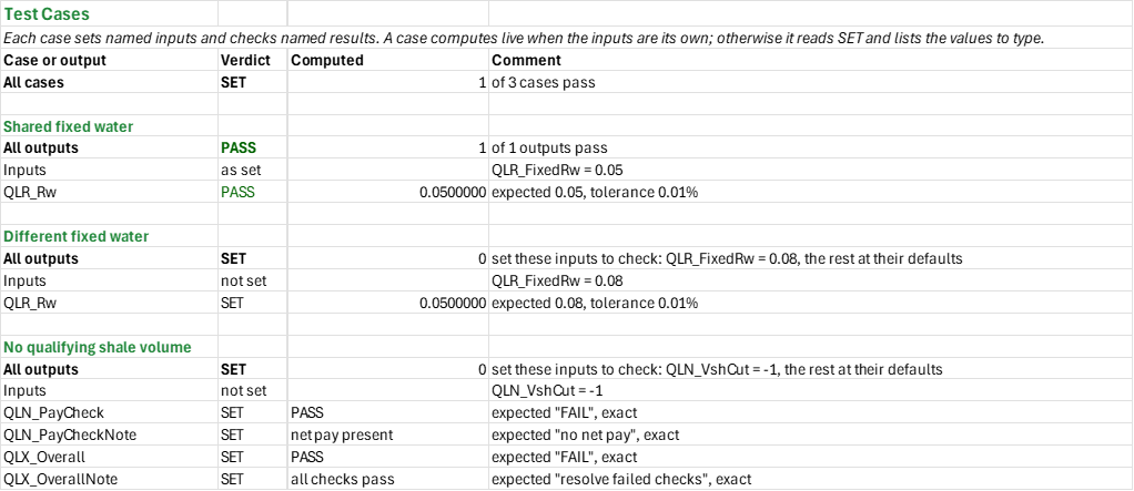
Guide— the workflow and which porosity feeds which calculation.Logs— the pasted log curves with the shale picks and porosity constants; shale volume by five transforms, density, neutron, density-neutron and sonic porosity, the zone porosity, and a depth track of shale volume and porosity.Water— formation-water resistivity from SP, minimum Rwa, Pickett and salinity, calibrated in the water sand, and the selected Rw.Saturation— Archie, Simandoux, Indonesia, Waxman-Smits and dual-water saturation over the selected window, with zone averages and a depth track.Pay— the cutoffs, the sample-by-sample reservoir and pay flags, gross, net reservoir and net pay, and a depth track of Vsh, porosity and Sw.Permeability— the core plugs on depth after the typed shift, Timur, Coates and Wyllie-Rose calibrated to the core, the core porosity-permeability fit, and the zone permeability.Summary— Rw, net pay, pay porosity, oil-zone permeability, the zone pay table and every check.Test Cases— the worked example and other cases, with expected and computed results.
Functions used
Names (192)
| Name | Refers to | Comment |
|---|---|---|
PO.PP.Cutoff.PermFromCoreLAMBDA |
=LAMBDA(Phi_core, K_core, K_cut, LET(lk, LOG10(K_core), b, SLOPE(lk, Phi_core), (LOG10(K_cut)-INTERCEPT(lk, Phi_core))/b)) |
Porosity cut-off at a permeability cut-off, from a least-squares fit of log10(k) on porosity to core points. |
PO.PP.Pay.NetPayLAMBDA |
=LAMBDA(H, Vsh, PhiEff_frac, Sw, Vsh_cut, Phi_cut, Sw_cut, LET(res, (Vsh<=Vsh_cut)*(PhiEff_frac>=Phi_cut), pay, res*(Sw<=Sw_cut), gross, SUM(H), net, SUM(H*res), np, SUM(H*pay), hp, SUM(H*PhiEff_frac*pay), HSTACK(gross, net, np, net/gross, IF(np>0, hp/np, 0), IF(hp>0, SUM(H*PhiEff_frac*Sw*pay)/hp, 0)))) |
Net reservoir and net pay over an interval from Vsh, porosity and Sw cut-offs: {gross, net reservoir, net pay, net-to-gross, pay porosity, pay Sw}. |
PO.PP.Perm.CoatesLAMBDA |
=LAMBDA(Phi, Swirr, 10000*Phi^4*((1-Swirr)/Swirr)^2) |
Coates free-fluid permeability, k = (100 phi^2 (1 - Swirr) / Swirr)^2, mD (fractions). |
PO.PP.Perm.PoroPermFitLAMBDA |
=LAMBDA(Phi_core, K_core, LET(lk, LOG10(K_core), HSTACK(INTERCEPT(lk, Phi_core), SLOPE(lk, Phi_core), RSQ(lk, Phi_core)))) |
Log-linear poro-perm transform fitted to core points, log10(k) = A + B phi: {A, B, R2}. |
PO.PP.Perm.TimurLAMBDA |
=LAMBDA(Phi, Swirr, 0.136*(100*Phi)^4.4/(100*Swirr)^2) |
Timur (1968) permeability, k = 0.136 phi^4.4 / Swirr^2 with phi and Swirr in percent, mD (arguments as fractions). |
PO.PP.Perm.WyllieRoseLAMBDA |
=LAMBDA(Phi, Swirr, Coef, Exp_Phi, Exp_Sw, Coef^2*Phi^(2*Exp_Phi)/Swirr^(2*Exp_Sw)) |
Wyllie-Rose (1950) general permeability form, k = (Coef phi^Exp_Phi / Swirr^Exp_Sw)^2, mD (fractions). |
PO.PP.Porosity.FromDensityLAMBDA |
=LAMBDA(Rho_ma, Rho_b, Rho_f, (Rho_ma-Rho_b)/(Rho_ma-Rho_f)) |
Porosity from a density log, (matrix density - bulk density) / (matrix density - fluid density). |
PO.PP.Porosity.FromNeutronDensityLAMBDA |
=LAMBDA(Phi_N, Phi_D, Mode, IF(Mode=1, (Phi_N+Phi_D)/2, IF(Mode=2, SQRT((Phi_N^2+Phi_D^2)/2), NA()))) |
Density-neutron crossplot porosity: Mode 1 the arithmetic mean (liquid-filled), Mode 2 the root-mean-square gas form sqrt((phiN^2 + phiD^2)/2). |
PO.PP.Porosity.FromSonic.RHGLAMBDA |
=LAMBDA(Dt, Dt_ma, C, C*(Dt-Dt_ma)/Dt) |
Raymer-Hunt-Gardner sonic porosity, C times (transit time minus matrix) over transit time. |
PO.PP.Porosity.FromSonic.WyllieLAMBDA |
=LAMBDA(Dt, Dt_ma, Dt_f, Dt_sh, ((Dt-Dt_ma)/(Dt_f-Dt_ma))/(Dt_sh/100)) |
Wyllie time-average sonic porosity divided by the shale compaction factor Dt_sh/100. |
PO.PP.Qv.FromCECLAMBDA |
=LAMBDA(CEC, PhiT_frac, Rho_g, CEC*(1-PhiT_frac)*Rho_g/(100*PhiT_frac)) |
Cation exchange capacity per unit pore volume, Qv = CEC (1 - phi) rho_g / (100 phi), meq/cm3, from CEC in meq/100 g. |
PO.PP.Rw.FromRwaLAMBDA |
=LAMBDA(Rt_ohmm, Phi_frac, a_tort, m_cem, MIN(Rt_ohmm*Phi_frac^m_cem/a_tort)) |
Rw as the minimum apparent water resistivity, Rwa = Rt phi^m / a, over a clean water-bearing interval. |
PO.PP.Rw.FromSalinityLAMBDA |
=LAMBDA(NaCl_ppm, 0.0123+3647.5/NaCl_ppm^0.955) |
NaCl solution resistivity at 75 degF from salinity in ppm, Rw75 = 0.0123 + 3647.5 / ppm^0.955 (the fitted form of the resistivity-salinity chart). |
PO.PP.Rw.FromSspLAMBDA |
=LAMBDA(SSP, Rmf_eq, T_F, Rmf_eq*10^(SSP/(61+0.133*T_F))) |
Equivalent formation-water resistivity from the static SP, for NaCl-dominant water. |
PO.PP.Rw.TemperatureLAMBDA |
=LAMBDA(R_ref, T_ref_F, T_F, R_ref*(T_ref_F+6.77)/(T_F+6.77)) |
Arps (1953) temperature correction of a water or mud resistivity, R = R_ref (T_ref + 6.77) / (T + 6.77), degF. |
PO.PP.Sw.ArchieLAMBDA |
=LAMBDA(a, m, n, Phi, Rw, Rt, ((a/Phi^m)*(Rw/Rt))^(1/n)) |
Water saturation from the general Archie equation, Sw = ((a/phi^m)*(Rw/Rt))^(1/n). |
PO.PP.Sw.DualWaterLAMBDA |
=LAMBDA(a, m, n, Phi_t, Rw, Rwb, Swb, Rt, Mode, LET(ct, 1/Rt, cw, 1/Rw, kf, Phi_t^m/a, bq, (1/Rwb-1/Rw)*Swb, swt, IF(Mode=1, IF(n=2, (-bq+SQRT(bq^2+4*cw*ct/kf))/(2*cw), NA()), IF(Mode=2, REDUCE(1, SEQUENCE(30), LAMBDA(s, j, s-(kf*(cw*s^n+bq*s^(n-1))-ct)/(kf*(n*cw*s^(n-1)+(n-1)*bq*s^(n-2))))), NA())), HSTACK(swt, (swt-Swb)/(1-Swb)))) |
Dual-water (Clavier et al. 1984) saturation: {Swt, Swe}. Mode 1 the quadratic closed form (n = 2 only), Mode 2 a 30-step Newton solve for any n. |
PO.PP.Sw.IndonesiaLAMBDA |
=LAMBDA(a, m, n, Phi_e, Rw, Rt, Vsh, Rsh, POWER(1/(SQRT(Rt)*(Vsh^(1-Vsh/2)/SQRT(Rsh)+Phi_e^(m/2)/SQRT(a*Rw))), 2/n)) |
Indonesia (Poupon-Leveaux 1971) water saturation for a shaly formation. |
PO.PP.Sw.SimandouxLAMBDA |
=LAMBDA(Phi_e, Rt, Rw, Vsh, Rsh, (0.4*Rw/Phi_e^2)*(-Vsh/Rsh+SQRT((Vsh/Rsh)^2+5*Phi_e^2/(Rw*Rt)))) |
Simandoux (1963) water saturation for a shaly sand, Bassiouni's a = 0.8 and m = 2 form. |
PO.PP.Sw.WaxmanSmitsLAMBDA |
=LAMBDA(a, m, n, Phi, Rw, Rt, B, Qv, Mode, LET(ct, 1/Rt, cw, 1/Rw, kf, Phi^m/a, bq, B*Qv, IF(Mode=1, IF(n=2, (-bq+SQRT(bq^2+4*cw*ct/kf))/(2*cw), NA()), IF(Mode=2, REDUCE(1, SEQUENCE(30), LAMBDA(s, j, s-(kf*(cw*s^n+bq*s^(n-1))-ct)/(kf*(n*cw*s^(n-1)+(n-1)*bq*s^(n-2))))), NA())))) |
Waxman-Smits (1968) water saturation from Qv and B: Mode 1 the quadratic closed form (n = 2 only), Mode 2 a 30-step Newton solve for any n. |
PO.PP.Vsh.ClavierLAMBDA |
=LAMBDA(IGR, 1.7-SQRT(3.38-(IGR+0.7)^2)) |
Clavier et al. (1971) shale volume from the gamma-ray index, Vsh = 1.7 - sqrt(3.38 - (IGR + 0.7)^2). |
PO.PP.Vsh.GammaRayIndexLAMBDA |
=LAMBDA(GR, GR_cl, GR_sh, (GR-GR_cl)/(GR_sh-GR_cl)) |
Linear gamma-ray shale index, IGR = (GR - GRclean) / (GRshale - GRclean). |
PO.PP.Vsh.Larionov.OlderLAMBDA |
=LAMBDA(IGR, 0.33*(2^(2*IGR)-1)) |
Larionov (1969) shale volume for older consolidated rocks, from the gamma-ray index. |
PO.PP.Vsh.Larionov.TertiaryLAMBDA |
=LAMBDA(IGR, 0.083*(2^(3.7*IGR)-1)) |
Larionov (1969) shale volume for Tertiary rocks, from the gamma-ray index. |
PO.PP.Vsh.SteiberLAMBDA |
=LAMBDA(IGR, IGR/(3-2*IGR)) |
Steiber (1970) shale volume from the gamma-ray index, Vsh = IGR / (3 - 2 IGR). |
QLA_BVW |
Summary!$B$35 |
Bulk volume water, v/v |
QLA_H |
Summary!$B$32 |
Clean oil-sand thickness, ft |
QLA_HCPT |
Summary!$B$36 |
Hydrocarbon pore thickness, ft |
QLA_Phi |
Summary!$B$33 |
Uncorrected density porosity, % |
QLA_RhoB |
Summary!$B$31 |
Clean oil-sand density, g/cm³ |
QLA_Rt |
Summary!$B$30 |
Clean oil-sand resistivity, ohm·m |
QLA_Sw |
Summary!$B$34 |
Archie water saturation, % |
QLK_A |
Permeability!$B$13 |
Core transform intercept |
QLK_B |
Permeability!$B$14 |
Core transform slope |
QLK_BiasC |
Permeability!$B$17 |
Coates bias, cycles |
QLK_BiasT |
Permeability!$B$16 |
Timur bias, cycles |
QLK_BiasW |
Permeability!$B$18 |
Wyllie-Rose bias, cycles |
QLK_Bvi |
Permeability!$B$4 |
Irreducible bulk volume water, v/v |
QLK_CalC |
Permeability!$B$20 |
Coates calibration |
QLK_CalT |
Permeability!$B$19 |
Timur calibration |
QLK_CalW |
Permeability!$B$21 |
Wyllie-Rose calibration |
QLK_Core |
Permeability!$A$41:$I$55 |
Core measurements and shifted log match |
QLK_DepthCheck |
Permeability!$B$28 |
Core depth and permeability verdict |
QLK_DepthCheckNote |
Permeability!$C$28 |
Core depth and permeability comment |
QLK_Inputs |
Permeability!$B$4:$B$11 |
Permeability calibration inputs |
QLK_KH |
Permeability!$B$26 |
Zone permeability thickness, mD·ft |
QLK_Log |
Permeability!$A$61:$J$106 |
Calibrated permeability by method |
QLK_Method |
Permeability!$B$11 |
Method (1 Timur, 2 Coates, 3 Wyllie-Rose, 4 core) |
QLK_MethodCheck |
Permeability!$B$29 |
Permeability method verdict |
QLK_MethodCheckNote |
Permeability!$C$29 |
Permeability method comment |
QLK_MethodCount |
Permeability!$B$32 |
Available permeability methods |
QLK_PhiMiss |
Permeability!$B$22 |
Core to log mean porosity miss, % |
QLK_PhiTol |
Permeability!$B$31 |
Core porosity match tolerance, % |
QLK_R2 |
Permeability!$B$15 |
Core transform R squared |
QLK_Results |
Permeability!$B$13:$B$29 |
Core transform and permeability results and checks |
QLK_Shift |
Permeability!$B$8 |
Core depth shift added to core depth, ft |
QLK_WrC |
Permeability!$B$5 |
Wyllie-Rose coefficient |
QLK_WrP |
Permeability!$B$6 |
Wyllie-Rose porosity exponent |
QLK_WrS |
Permeability!$B$7 |
Wyllie-Rose Swirr exponent |
QLK_ZBase |
Permeability!$B$10 |
Zone base, ft |
QLK_ZK |
Permeability!$B$25 |
Zone permeability, mD |
QLK_ZPhi |
Permeability!$B$23 |
Zone porosity, % |
QLK_ZSwi |
Permeability!$B$24 |
Zone Swirr, % |
QLK_ZTop |
Permeability!$B$9 |
Zone top, ft |
QLN_Base |
Pay!$B$5 |
Gross interval base, ft |
QLN_GPhi |
Pay!$B$13 |
Gross mean corrected density porosity, % |
QLN_GSw |
Pay!$B$14 |
Gross mean Archie Sw, % |
QLN_GVsh |
Pay!$B$12 |
Gross mean Vsh, v/v |
QLN_Gross |
Pay!$B$15 |
Gross thickness, ft |
QLN_Inputs |
Pay!$B$4:$B$9 |
Interval and cutoffs |
QLN_KCut |
Pay!$B$9 |
Core permeability cutoff, mD |
QLN_Log |
Pay!$A$41:$G$101 |
Sample thickness and cutoffs |
QLN_NTG |
Pay!$B$18 |
Net to gross, % |
QLN_NTGIndex |
Pay!$B$26 |
Net-to-gross result index |
QLN_Net |
Pay!$B$16 |
Net reservoir, ft |
QLN_Pay |
Pay!$B$17 |
Net pay, ft |
QLN_PayCheck |
Pay!$B$23 |
Net pay verdict |
QLN_PayCheckNote |
Pay!$C$23 |
Net pay comment |
QLN_PayIndex |
Pay!$B$25 |
Net-pay result index |
QLN_PayPhi |
Pay!$B$19 |
Pay mean corrected density porosity, % |
QLN_PaySw |
Pay!$B$20 |
Pay mean water saturation, % |
QLN_PhiCore |
Pay!$B$21 |
Core-derived porosity cutoff, % |
QLN_PhiCut |
Pay!$B$7 |
Minimum corrected density porosity, % |
QLN_PhiIndex |
Pay!$B$27 |
Pay porosity result index |
QLN_Results |
Pay!$B$11:$B$23 |
Gross and net pay |
QLN_Step |
Pay!$B$11 |
Sample spacing, ft |
QLN_SwCut |
Pay!$B$8 |
Maximum water saturation, % |
QLN_SwIndex |
Pay!$B$28 |
Pay saturation result index |
QLN_Top |
Pay!$B$4 |
Gross interval top, ft |
QLN_VshCut |
Pay!$B$6 |
Maximum shale volume, v/v |
QLP_C |
Logs!$B$13 |
RHG coefficient |
QLP_DtF |
Logs!$B$12 |
Fluid transit time, µs/ft |
QLP_DtMa |
Logs!$B$11 |
Matrix transit time, µs/ft |
QLP_DtSh |
Logs!$B$10 |
Shale sonic transit time, µs/ft |
QLP_GRcl |
Logs!$B$4 |
Clean gamma ray, API |
QLP_GRsh |
Logs!$B$5 |
Shale gamma ray, API |
QLP_GasX |
Logs!$B$14 |
Density-neutron crossover, % |
QLP_Inputs |
Logs!$B$4:$B$17 |
Log interpretation inputs |
QLP_Log |
Logs!$A$32:$S$92 |
Shared input curves and derived shale and porosity curves |
QLP_NphiSh |
Logs!$B$9 |
Shale neutron porosity, % |
QLP_PhiDsh |
Logs!$B$18 |
Shale density porosity, % |
QLP_PhiND |
Logs!$B$21 |
Zone corrected density-neutron, % |
QLP_PhiRsh |
Logs!$B$20 |
Shale RHG porosity, % |
QLP_PhiWsh |
Logs!$B$19 |
Shale Wyllie porosity, % |
QLP_PicksCheck |
Logs!$B$23 |
Gamma ray picks verdict |
QLP_PicksCheckNote |
Logs!$C$23 |
Gamma ray picks comment |
QLP_Results |
Logs!$B$18:$B$24 |
Porosity results and checks |
QLP_RhoF |
Logs!$B$7 |
Fluid density, g/cm³ |
QLP_RhoMa |
Logs!$B$6 |
Matrix density, g/cm³ |
QLP_RhoSh |
Logs!$B$8 |
Shale density, g/cm³ |
QLP_WindowCheck |
Logs!$B$24 |
Log spacing and window verdict |
QLP_WindowCheckNote |
Logs!$C$24 |
Log spacing and window comment |
QLP_WindowCount |
Logs!$B$94 |
Window samples |
QLP_WindowStart |
Logs!$B$22 |
Window start row in log |
QLP_WindowTop |
Logs!$B$17 |
Saturation and permeability window top, ft |
QLP_ZBase |
Logs!$B$16 |
Porosity zone base, ft |
QLP_ZTop |
Logs!$B$15 |
Porosity zone top, ft |
QLR_FixedRw |
Water!$B$16 |
Fixed Rw at formation temperature, ohm·m |
QLR_Inputs |
Water!$B$4:$B$16 |
Electrical parameters and water sample |
QLR_Log |
Water!$A$41:$G$101 |
Shared logs and water-sand flag |
QLR_Method |
Water!$B$15 |
Rw source (1 SP, 2 Rwa, 3 Pickett, 4 salinity, 5 fixed) |
QLR_MethodCount |
Water!$B$32 |
Available Rw methods |
QLR_Ppm |
Water!$B$14 |
Water salinity, ppm |
QLR_Results |
Water!$B$18:$B$30 |
Rw estimates and selection |
QLR_Rmf |
Water!$B$9 |
Filtrate resistivity at reference temperature, ohm·m |
QLR_RmfT |
Water!$B$19 |
Filtrate at formation temperature, ohm·m |
QLR_Rmfe |
Water!$B$20 |
Equivalent filtrate resistivity, ohm·m |
QLR_RmfeK |
Water!$B$10 |
Equivalent filtrate factor |
QLR_Rw |
Water!$B$28 |
Selected Rw, ohm·m |
QLR_RwPk |
Water!$B$25 |
Pickett Rw, ohm·m |
QLR_RwRef |
Water!$B$26 |
Rw at reference temperature from salinity, ohm·m |
QLR_RwRwa |
Water!$B$24 |
Minimum Rwa, ohm·m |
QLR_RwSP |
Water!$B$23 |
Rw from SP, ohm·m |
QLR_RwSal |
Water!$B$27 |
Rw from salinity at formation temperature, ohm·m |
QLR_SPsh |
Water!$B$11 |
Shale SP baseline, mV |
QLR_SSP |
Water!$B$22 |
Static SP, mV |
QLR_Tf |
Water!$B$7 |
Formation temperature, °F |
QLR_Tref |
Water!$B$8 |
Reference temperature, °F |
QLR_WBase |
Water!$B$13 |
Water sand base, ft |
QLR_WPhi |
Water!$B$18 |
Mean water-sand porosity, % |
QLR_WSP |
Water!$B$21 |
Water sand mean SP, mV |
QLR_WTop |
Water!$B$12 |
Water sand top, ft |
QLR_WaterCheck |
Water!$B$30 |
Water inputs verdict |
QLR_WaterCheckNote |
Water!$C$30 |
Water inputs comment |
QLR_a |
Water!$B$4 |
Tortuosity |
QLR_m |
Water!$B$5 |
Cementation exponent |
QLR_n |
Water!$B$6 |
Saturation exponent |
QLS_B |
Saturation!$B$14 |
Juhasz clay conductance, (S/m)/(meq/cm³) |
QLS_CECsh |
Saturation!$B$5 |
Shale cation exchange capacity, meq/100 g |
QLS_Inputs |
Saturation!$B$4:$B$9 |
Shale parameters |
QLS_J1 |
Saturation!$B$81 |
Juhasz constant term |
QLS_J2 |
Saturation!$B$82 |
Juhasz temperature term |
QLS_J3 |
Saturation!$B$83 |
Juhasz temperature-squared term |
QLS_J4 |
Saturation!$B$84 |
Juhasz Rw exponent |
QLS_J5 |
Saturation!$B$85 |
Juhasz Rw temperature slope |
QLS_J6 |
Saturation!$B$86 |
Juhasz Rw constant |
QLS_Log |
Saturation!$A$31:$N$76 |
Saturation models over the source interval |
QLS_Mode |
Saturation!$B$15 |
Solve mode |
QLS_PhiCut |
Saturation!$B$9 |
Reservoir effective porosity cutoff, % |
QLS_PhiTsh |
Saturation!$B$11 |
Shale density porosity, % |
QLS_Results |
Saturation!$B$11:$B$23 |
Shaly model zone results |
QLS_Rsh |
Saturation!$B$4 |
Shale resistivity, ohm·m |
QLS_Rwb |
Saturation!$B$12 |
Bound-water resistivity, ohm·m |
QLS_ShaleCheck |
Saturation!$B$23 |
Shale inputs verdict |
QLS_ShaleCheckNote |
Saturation!$C$23 |
Shale inputs comment |
QLS_TfC |
Saturation!$B$13 |
Formation temperature (C), °C |
QLS_TfPerC |
Saturation!$B$80 |
Fahrenheit degrees per Celsius degree |
QLS_TfZero |
Saturation!$B$79 |
Water freezing point (F), °F |
QLS_VshCut |
Saturation!$B$8 |
Reservoir Vsh cutoff, v/v |
QLS_ZBase |
Saturation!$B$7 |
Shaly oil zone base, ft |
QLS_ZSwA |
Saturation!$B$17 |
Zone Archie, effective, % |
QLS_ZSwD |
Saturation!$B$21 |
Zone dual water, % |
QLS_ZSwI |
Saturation!$B$19 |
Zone Indonesia, % |
QLS_ZSwS |
Saturation!$B$18 |
Zone Simandoux, % |
QLS_ZSwT |
Saturation!$B$22 |
Zone Archie, total, % |
QLS_ZSwW |
Saturation!$B$20 |
Zone Waxman-Smits, % |
QLS_ZSwb |
Saturation!$B$16 |
Zone mean bound water, % |
QLS_ZTop |
Saturation!$B$6 |
Shaly oil zone top, ft |
QLV_IGR |
Logs!$B$28 |
Zone gamma-ray index, v/v |
QLV_LarT |
Logs!$B$29 |
Zone Larionov Tertiary, v/v |
QLV_ZBase |
Logs!$B$26 |
Vsh zone base, ft |
QLV_ZTop |
Logs!$B$25 |
Vsh zone top, ft |
QLV_ZoneGR |
Logs!$B$27 |
Zone mean gamma ray, API |
QLX_Checks |
Summary!$B$12:$B$18 |
All checks |
QLX_K |
Summary!$B$7 |
Oil-zone calibrated permeability, mD |
QLX_Overall |
Summary!$B$10 |
Overall interpretation verdict |
QLX_OverallNote |
Summary!$C$10 |
Overall interpretation comment |
QLX_Pay |
Summary!$B$5 |
Interval net pay, ft |
QLX_PayPhi |
Summary!$B$6 |
Pay corrected density porosity, % |
QLX_Results |
Summary!$B$4:$B$10 |
Results and overall verdict |
QLX_Rw |
Summary!$B$4 |
Selected formation-water resistivity, ohm·m |
QLX_Zones |
Summary!$A$21:$D$25 |
Zone net pay using corrected density porosity and Archie saturation |
Details
| Opens in | Needs Microsoft 365 or Excel 2024: it uses functions Excel 2016 doesn't have, such as named LAMBDAs, which show #NAME? there. |
| File | QuickLookInterpretation.xlsx, 129 KB |
| Category | Petrophysics |
| For agents and tools | Descriptor (.md) |