Rate-Transient Analysis and Flowing Material Balance
Description
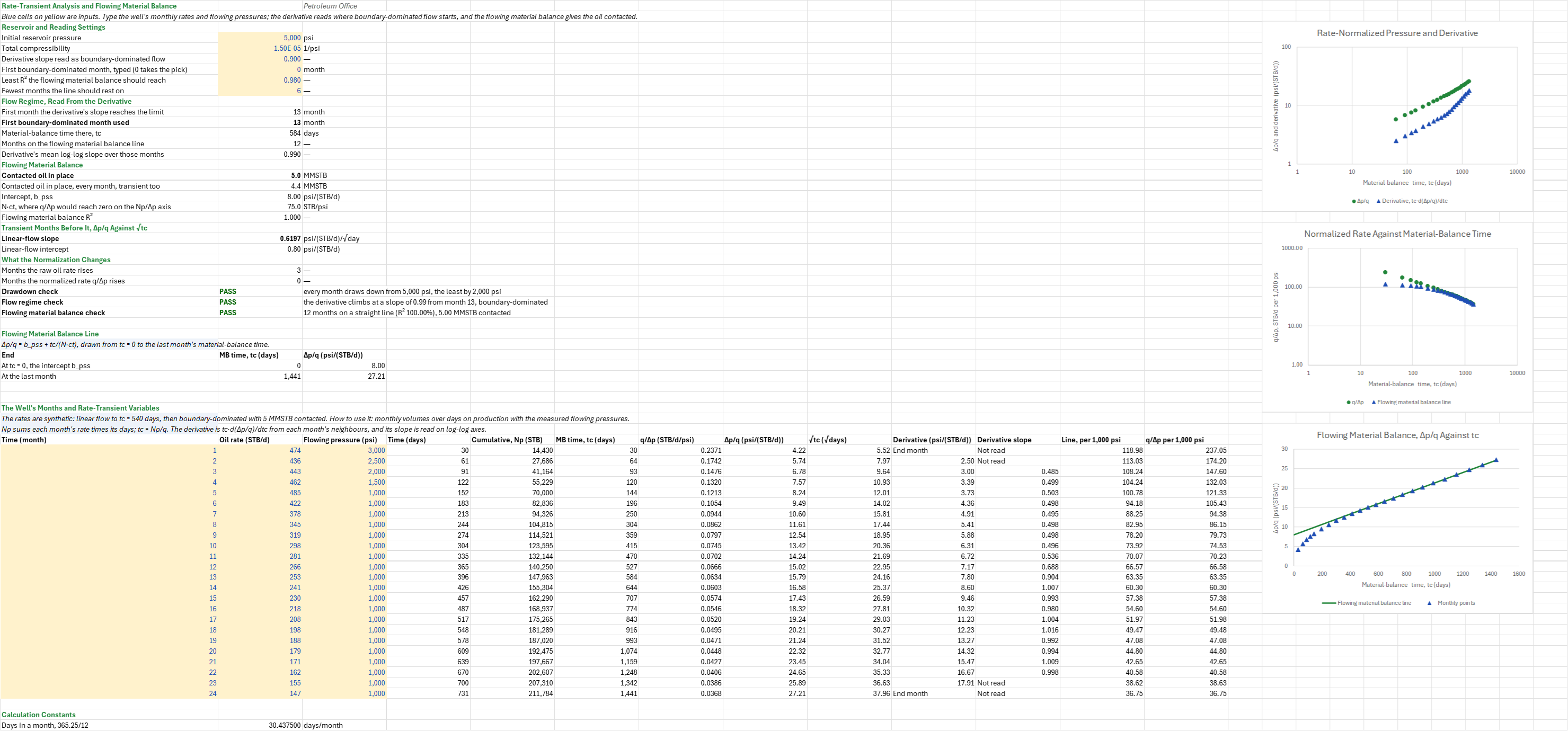
How much oil has the well contacted, and is there enough data to say? You enter the initial reservoir pressure, the total compressibility and each month's oil rate and flowing bottomhole pressure. The sheet sets each rate, normalized by its drawdown, against material-balance time, so a well whose flowing pressure changed reads as if it had produced at one rate. You read off the flow regime month by month, the first boundary-dominated month and the oil in place the well has contacted.
Parameters:
- Reservoir: the initial reservoir pressure
FMB_Pi(psi) and the total compressibilityFMB_Ct(1/psi) - Reading: the derivative slope read as boundary-dominated
FMB_SlopeBdf, and a typed first boundary-dominated monthFMB_MUser(0 takes the sheet's pick) - Line: the least R²
FMB_R2Minand the fewest monthsFMB_MinPtsthe line should rest on - Months: the oil rate (STB/d) and flowing bottomhole pressure (psi) of each of 24 months
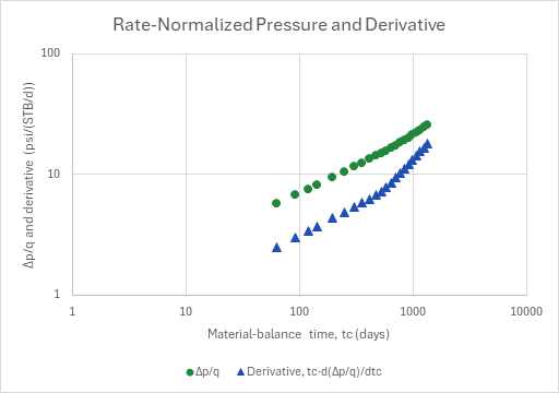
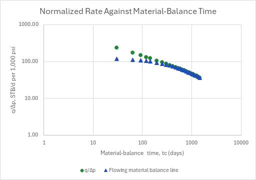
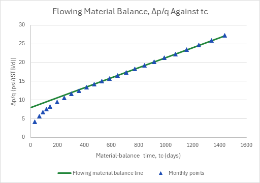
How to use it: Compute monthly rates as each month's volume over its days on production, type the bottomhole flowing pressure of each month (gauge, or computed from the wellhead), and take out shut-in and partial months first (the Production Data Cleaning sheet). The rate-normalized pressure Δp/q and its derivative go on log-log axes: the derivative rises at a slope of ½ in linear flow and of 1 once the well feels its boundaries. The sheet reads that slope month by month and picks the first boundary-dominated month; read the derivative over several months, not one, and type the pick by hand when the derivative is noisy. Check that every month draws down enough, that the months after the pick are boundary-dominated, and that the flowing material balance line is straight over enough months. Then read the contacted oil in place with b_pss, N·ct and R², and the √tc line of the transient months before the pick. Three charts draw the diagnostic, the normalized rate against tc with the line's q/Δp (both per 1,000 psi of drawdown, so the log axis starts above 1), and the flowing material balance itself.
Method: Time is the month times 365.25/12 days. Np is cumulated month by month as each month's rate times its days, and material-balance time is tc = Np/q. The normalized rate is q/Δp = q/(pi − pwf), and Δp/q is its inverse. The derivative tc·d(Δp/q)/dtc at a month is Bourdet's three-point form in x = ln tc with its two neighbours, ((Δy₁/Δx₁)·Δx₂ + (Δy₂/Δx₂)·Δx₁)/(Δx₁ + Δx₂), so the first and last months have none. Its log-log slope at a month is ln(d₊/d₋)/ln(tc₊/tc₋) over the two neighbours, read from month 3 to month 22. In linear flow Δp/q = b + m·√tc and the derivative is (m/2)·√tc, a slope of ½; in boundary-dominated flow Δp/q = b_pss + tc/(N·ct) and the derivative is tc/(N·ct), a slope of 1. The pick is the first month whose slope reaches the boundary-dominated slope you set. The flowing material balance takes the months from the one used and fits Δp/q against tc by least squares: N = 1/(slope·ct), with b_pss the intercept and N·ct the line's reach on the Agarwal-Gardner Np/Δp axis. The months before it give the √tc line by Excel's SLOPE and INTERCEPT.
Example: The default is a tight-oil horizontal in the decline family's reservoir (5,000 psi, 1.5 × 10⁻⁵ 1/psi, the Decline and Flow-Regime Diagnostics sheet's), whose flowing pressure was drawn down from 3,000 to 1,000 psi over its first five months and then held. Its rates are synthetic. The well's constant-rate response is linear flow, Δp/q = 0.8 + 0.6197·√t, to t = 540 days, then boundary-dominated, Δp/q = 8 + t/75, with N = 5 MMSTB and N·ct = 75 STB/psi; the slope 0.6197 = 2·√540/75 joins the two in value and in slope. Each month's rate puts its point on that response in material-balance time at that month's pressure, to a tenth of a barrel. So the raw rate rises from 435.5 to 485.3 STB/d over months 2 to 5, while q/Δp falls every month.
The derivative's slope reads 0.48 to 0.50 over months 3 to 10, 0.54 and 0.69 at months 11 and 12, and 0.90 at month 13 (tc = 584 days), so the pick is month 13. The 12 months from there climb at a mean slope of 0.99: boundary-dominated. Over them the flowing material balance is a straight line (R² 1.0000) with b_pss = 7.999 psi/(STB/d) and N·ct = 75.00 STB/psi, so N = 75.00/1.5 × 10⁻⁵ = 5.00 MMSTB contacted. Over every month, linear flow included, it would be 4.38 MMSTB: transient months pull the volume down. The 12 transient months lie on Δp/q = 0.7999 + 0.6197·√tc, the response the rates were built on. The raw rate rises in 3 months and q/Δp in none, and every month draws down by at least 2,000 psi.
Functions used
None: the blueprint calculates with Excel's own functions.
Names (43)
| Name | Refers to | Comment |
|---|---|---|
PO.RTA.NormalizedRateLAMBDA |
=LAMBDA(q, p_i, p_wf, IF((q<=0)+(p_i<=p_wf), NA(), q/(p_i-p_wf))) |
Pressure-normalized rate q/(p_i - p_wf), STB/d/psi: the rate over the drawdown from the initial reservoir pressure. Works on single values or whole columns. For gas pass pseudo-pressures m(p_i), m(p_wf). |
PO.RTA.FlowingMBLAMBDA |
=LAMBDA(n_p, q, p_i, p_wf, ct, IF((ct<=0)+(SLOPE((p_i-p_wf)/q, n_p/q)<=0), NA(), 1/(SLOPE((p_i-p_wf)/q, n_p/q)*ct))) |
Contacted oil in place, STB, by flowing material balance: fits (p_i - p_wf)/q against material-balance time Np/q and returns 1/(slope*ct). Np in STB, q in STB/d, pressures in psi, ct in 1/psi; boundary-dominated points only. |
FMB_Pi |
$B$4 |
Initial reservoir pressure, psi |
FMB_Ct |
$B$5 |
Total compressibility, 1/psi |
FMB_SlopeBdf |
$B$6 |
Derivative slope read as boundary-dominated flow |
FMB_MUser |
$B$7 |
First boundary-dominated month, typed (0 takes the pick), month |
FMB_R2Min |
$B$8 |
Least R² the flowing material balance should reach |
FMB_MinPts |
$B$9 |
Fewest months the line should rest on |
FMB_Inputs |
$B$4:$B$9 |
The initial reservoir pressure, the total compressibility, the derivative slope read as boundary-dominated, a typed first boundary-dominated month, the least R² and the fewest months for the line |
FMB_MPick |
$B$11 |
First month the derivative's slope reaches the limit, month |
FMB_MBdf |
$B$12 |
First boundary-dominated month used, month |
FMB_TcBdf |
$B$13 |
Material-balance time there, tc, days |
FMB_NBdf |
$B$14 |
Months on the flowing material balance line |
FMB_SlopeLate |
$B$15 |
Derivative's mean log-log slope over those months |
FMB_OOIP |
$B$17 |
Contacted oil in place, MMSTB |
FMB_OOIPAll |
$B$18 |
Contacted oil in place, every month, transient too, MMSTB |
FMB_Bpss |
$B$19 |
Intercept, b_pss, psi/(STB/d) |
FMB_NCt |
$B$20 |
N·ct, where q/Δp would reach zero on the Np/Δp axis, STB/psi |
FMB_FmbR2 |
$B$21 |
Flowing material balance R² |
FMB_LinSlope |
$B$23 |
Linear-flow slope, psi/(STB/d)/√day |
FMB_LinInt |
$B$24 |
Linear-flow intercept, psi/(STB/d) |
FMB_QRise |
$B$26 |
Months the raw oil rate rises |
FMB_NRise |
$B$27 |
Months the normalized rate q/Δp rises |
FMB_PressureCheck |
$B$28 |
Drawdown check verdict |
FMB_PressureCheckNote |
$C$28 |
Drawdown check comment |
FMB_RegimeCheck |
$B$29 |
Flow regime check verdict |
FMB_RegimeCheckNote |
$C$29 |
Flow regime check comment |
FMB_LineCheck |
$B$30 |
Flowing material balance check verdict |
FMB_LineCheckNote |
$C$30 |
Flowing material balance check comment |
FMB_Results |
$B$11:$B$30 |
Derivative's boundary-dominated onset, month used, its material-balance time, months on the line, their derivative log-log slope, contacted OIP over them and all months, b_pss, N·ct, R², transient √tc line, months raw and normalized rates rise, 3 checks |
FMB_Line |
$A$35:$C$36 |
The flowing material balance line, Δp/q = b_pss + tc/(N·ct), at tc = 0 and at the last month's material-balance time |
FMB_History |
$A$43:$M$66 |
Each month's time, oil rate and flowing pressure, time in days, cumulative and material-balance time, normalized rate and inverse, √tc, the derivative of Δp/q in ln tc and its log-log slope, and the FMB line's and measured q/Δp in STB/d per 1,000 psi |
FMB_T |
$A$43:$A$66 |
Months, 1 to 24 |
FMB_Q |
$B$43:$B$66 |
Oil rates, STB/d |
FMB_Pwf |
$C$43:$C$66 |
Flowing bottomhole pressures, psi |
FMB_Np |
$E$43:$E$66 |
Cumulative oil to each month, STB |
FMB_Tc |
$F$43:$F$66 |
Material-balance time Np/q, days |
FMB_Rnp |
$H$43:$H$66 |
Rate-normalized pressure (pi - pwf)/q, psi/(STB/d) |
FMB_RootTc |
$I$43:$I$66 |
Square root of material-balance time, √days |
FMB_Curve |
$F$44:$J$65 |
Rate-Normalized Pressure and Derivative |
FMB_Rate_Curve |
$F$43:$M$66 |
Normalized Rate Against Material-Balance Time |
FMB_Fmb_Curve |
$B$35:$H$36 |
Flowing Material Balance, Δp/q Against tc |
FMB_DMo |
$B$69 |
Days in a month, 365.25/12, days/month |
Details
| Inserts | 69 rows × 13 columns |
| Category | Decline Curve Analysis |
| For agents and tools | Descriptor (.md) |