Relative Permeability Fit by LINEST
Description
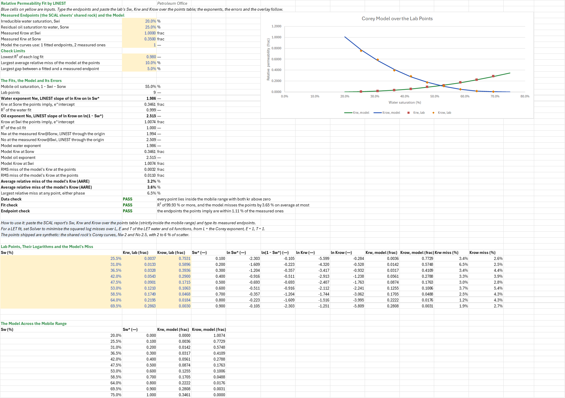
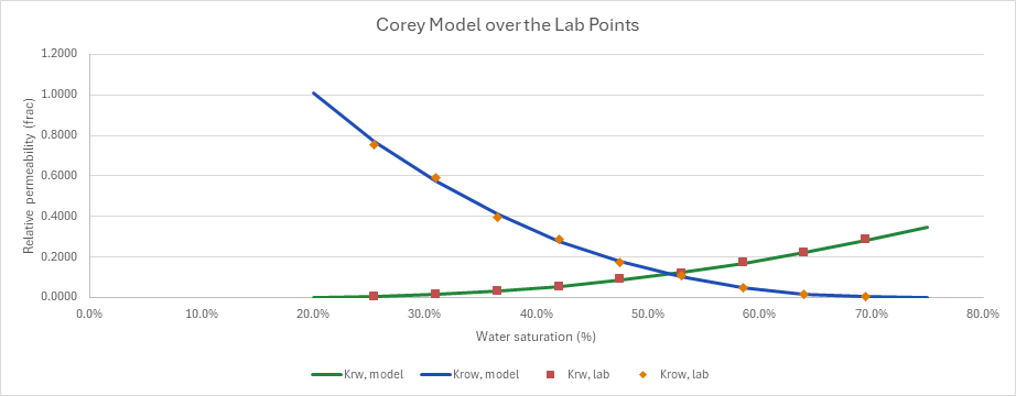
How well does a Corey model hold a set of lab water-oil relative permeability points, and what endpoints do the points imply? You enter the measured endpoints, the lab Sw, Krw and Krow, and which model to use. You read off each Corey exponent and implied endpoint from LINEST on the logarithms, the exponents through the measured endpoints, the R², RMS, average and largest misses, three checks on the data, the fit and the endpoints, and the model curves over the lab points.
Parameters:
- Measured endpoints: irreducible water saturation
RPF_Swi, residual oil saturation to waterRPF_Sorw, Krow at SwiRPF_KroEndand Krw at SorwRPF_KrwEnd - Model:
RPF_Mode, 1 for the fitted endpoints and exponents, 2 for the measured endpoints with the exponents fitted through them - Lab points: Sw, Krw and Krow at each point, the
RPF_Pointstable (namedRPF_Sw,RPF_KrwandRPF_Krow) - Check limits: the lowest R² of each log fit
RPF_R2Min(0.98), the largest average relative missRPF_AareMax(10 %), and the largest gap between a fitted and a measured endpointRPF_EndTol(5 %)
How to use it: Paste the SCAL report's Sw, Krw and Krow over the points table, using points strictly between Swi and 1 − Sorw with both kr above zero (the fit takes logarithms), and type the report's measured endpoints. Choose the model: the free fit's endpoints and exponents, or the measured endpoints with the exponents fitted through them. Where the SCAL Endpoint Analysis sheet averages several plugs' endpoints and fits the exponents through them, this sheet lets the points speak for their own endpoints and reports the errors. If one Corey exponent doesn't hold the points (the fit check warns), fit LET instead; the sheet ships no Solver model. Set Solver to minimise the sum of squared log misses, Σ (ln kr − ln kr(LET))², over L, E and T of the LET water and oil functions, starting from L = the Corey exponent, E = 1 and T = 1, inside Lomeland's bounds (L ≥ 1, E > 0, T ≥ 0.5). Type the model's exponents and endpoints into the SCAL Tables Export sheet for the simulator keywords.
Method:
- Normalised saturation. Sw* = (Sw − Swi)/(1 − Swi − Sorw) on the measured Swi and Sorw.
- Free fit. Corey's Krw = Krw@Sorw·Sw*^Nw and Krow = Krow@Swi·(1 − Sw*)^No are straight lines in logarithms: ln Krw = ln Krw@Sorw + Nw·ln Sw*, and ln Krow = ln Krow@Swi + No·ln(1 − Sw*).
INDEX(LINEST(ln Krw, ln Sw*), 1)is Nw andEXP(INDEX(…, 2))the Krw@Sorw the points imply; likewise for oil. R² isRSQon the same logarithms. - Through the measured endpoints.
LINEST(ln Krw − ln Krw@Sorw, ln Sw*, FALSE)fits the same line with no intercept, so its slope is the exponent at the measured endpoint, Σxy/Σx². - Model and errors. Corey on the chosen pair, written in the cells at each point and across the mobile range: the catalog's Corey functions refuse an endpoint above 1, and a free fit can imply one (1.0074 here). The RMS miss is √(Σ (model − lab)²/n), the average relative miss (AARE) the mean of |model/lab − 1|, and the largest miss the largest |model/lab − 1| of either phase. A fit in logarithms weighs each point by its relative miss, as the log scales a SCAL report is read on do.
- Checks. Data: fails for a model other than 1 or 2, a point outside the open mobile range or with a kr of zero, or fewer than three points. Fit: both R² at least the lowest R² and both AARE at most the largest average miss, else a warning that one exponent doesn't hold the points. Endpoints: the free fit's Krw@Sorw and Krow@Swi within the endpoint tolerance of the measured ones.
Example: The defaults are the rock the SCAL sheets share: a water-wet sandstone with Swi 20 %, Sorw 25 %, Krow@Swi 1 and Krw@Sorw 0.35, whose Corey exponents are Nw 2 and No 2.5. The nine lab points are synthetic: that rock's curves at Sw* = 0.1, 0.2, … 0.9 (Sw 25.5 % to 69.5 %), each given 2 to 6 % of scatter and read to four places. The free fit gives Nw = 1.9859 with a Krw@Sorw of 0.3461 (R² 0.99934), and No = 2.5147 with a Krow@Swi of 1.0074 (R² 0.99951), close to the 2 and 2.5 the points were built from. Through the measured endpoints the exponents are 1.9938 and 2.5094. The free model misses Krw by 0.0032 and Krow by 0.0110 RMS, 3.22 % and 3.65 % on average, and 6.49 % at worst (Krw at the second point, Sw 31 %, where the lab reads 0.0133 and the model 0.0142). The endpoints the points imply are within 1.11 % of the measured ones.
Functions used
None: the blueprint calculates with Excel's own functions.
Names (48)
| Name | Refers to | Comment |
|---|---|---|
RPF_Swi |
$B$4 |
Irreducible water saturation, Swi, % |
RPF_Sorw |
$B$5 |
Residual oil saturation to water, Sorw, % |
RPF_KroEnd |
$B$6 |
Measured Krow at Swi, frac |
RPF_KrwEnd |
$B$7 |
Measured Krw at Sorw, frac |
RPF_Mode |
$B$8 |
Model the curves use: 1 fitted endpoints, 2 measured ones |
RPF_R2Min |
$B$10 |
Lowest R² of each log fit |
RPF_AareMax |
$B$11 |
Largest average relative miss of the model at the points, % |
RPF_EndTol |
$B$12 |
Largest gap between a fitted and a measured endpoint, % |
RPF_Inputs |
$B$4:$B$12 |
The measured endpoints, the model the curves use, and the R², average-miss and endpoint limits of the checks |
RPF_Mobile |
$B$15 |
Mobile oil saturation, 1 − Swi − Sorw, % |
RPF_NPts |
$B$16 |
Lab points |
RPF_Nw |
$B$17 |
Water exponent Nw, LINEST slope of ln Krw on ln Sw* |
RPF_KrwFit |
$B$18 |
Krw at Sorw the points imply, e^intercept, frac |
RPF_R2w |
$B$19 |
R² of the water fit |
RPF_No |
$B$20 |
Oil exponent No, LINEST slope of ln Krow on ln(1 − Sw*) |
RPF_KroFit |
$B$21 |
Krow at Swi the points imply, e^intercept, frac |
RPF_R2o |
$B$22 |
R² of the oil fit |
RPF_NwFix |
$B$23 |
Nw at the measured Krw@Sorw, LINEST through the origin |
RPF_NoFix |
$B$24 |
No at the measured Krow@Swi, LINEST through the origin |
RPF_UseNw |
$B$25 |
Model water exponent |
RPF_UseKrw |
$B$26 |
Model Krw at Sorw, frac |
RPF_UseNo |
$B$27 |
Model oil exponent |
RPF_UseKro |
$B$28 |
Model Krow at Swi, frac |
RPF_RmseW |
$B$29 |
RMS miss of the model's Krw at the points, frac |
RPF_RmseO |
$B$30 |
RMS miss of the model's Krow at the points, frac |
RPF_AareW |
$B$31 |
Average relative miss of the model's Krw (AARE), % |
RPF_AareO |
$B$32 |
Average relative miss of the model's Krow (AARE), % |
RPF_MaxMiss |
$B$33 |
Largest relative miss at any point, either phase, % |
RPF_DataCheck |
$B$34 |
Data check verdict |
RPF_DataCheckNote |
$C$34 |
Data check comment |
RPF_FitCheck |
$B$35 |
Fit check verdict |
RPF_FitCheckNote |
$C$35 |
Fit check comment |
RPF_EndCheck |
$B$36 |
Endpoint check verdict |
RPF_EndCheckNote |
$C$36 |
Endpoint check comment |
RPF_Results |
$B$15:$B$36 |
The mobile range and point count; the free fits' exponents, endpoints and R²; the exponents through the measured endpoints; the model's four parameters; its RMS and average misses and the largest; and three checks |
RPF_Points |
$A$44:$L$52 |
Each lab point's Sw, Krw and Krow, its normalised saturation and the logarithms the fits take, the model's Krw and Krow there and the relative misses |
RPF_Sw |
$A$44:$A$52 |
Lab water saturations |
RPF_Krw |
$B$44:$B$52 |
Lab Krw |
RPF_Krow |
$C$44:$C$52 |
Lab Krow |
RPF_LnS |
$E$44:$E$52 |
ln Sw* of each point |
RPF_Ln1S |
$F$44:$F$52 |
ln(1 - Sw*) of each point |
RPF_LnKrw |
$G$44:$G$52 |
ln Krw of each point |
RPF_LnKrow |
$H$44:$H$52 |
ln Krow of each point |
RPF_KrwMod |
$I$44:$I$52 |
Model Krw at each point |
RPF_KroMod |
$J$44:$J$52 |
Model Krow at each point |
RPF_MissW |
$K$44:$K$52 |
Relative miss of the model Krw at each point |
RPF_MissO |
$L$44:$L$52 |
Relative miss of the model Krow at each point |
RPF_Curve |
$A$57:$D$67 |
Sw from Swi to 1 − Sorw, Sw*, and the model's Krw and Krow |
Details
| Inserts | 67 rows × 12 columns |
| Category | Special Core Analysis |
| For agents and tools | Descriptor (.md) |