Gas Buildup in Pseudo-Pressure
Description
What permeability, mechanical skin and rate-dependent skin does a gas well show in two buildups after two rates? You paste each buildup's shut-in times and pressures and set the rates, the flow time, the gas and the rock. The sheet reads each buildup in the real-gas pseudo-pressure m(p) against pseudo-time, which make the gas flow equation behave like a liquid's, and fits its Horner line for k and the apparent skin S′. You read off k, the mechanical skin S and the rate-dependent coefficient D.
Parameters:
- Reservoir, gas and well: pi, T, the gas gravity, h, φ, Swi, the rock and water compressibility, rw and the base pressure of m(p) (
GPB_Pi,GPB_T,GPB_SG,GPB_h,GPB_phi,GPB_Swi,GPB_cf,GPB_rw,GPB_Pbase) - The two buildups: the two rates, the flow time before each, and the flowing pressure at each shut-in (
GPB_q1,GPB_q2,GPB_tp,GPB_Pwf1,GPB_Pwf2; 0 takes the model's) - Analysis settings: the Bourdet window (
GPB_L, 0.2), the radial-flow window in pseudo-time (GPB_From,GPB_To, 2.37 to 23.7 hr), how flat the derivative must be over it (GPB_Flat, ±10 %), and the round-trip tolerance on k and D (GPB_Tol, ±5 %) - Synthetic model: k, S, D and the wellbore storage coefficient the buildups are made from (
GPB_ModelK,GPB_ModelS,GPB_ModelD,GPB_C) - Shut-in data: Δt and pws of each buildup, the regions
GPB_Data1andGPB_Data2
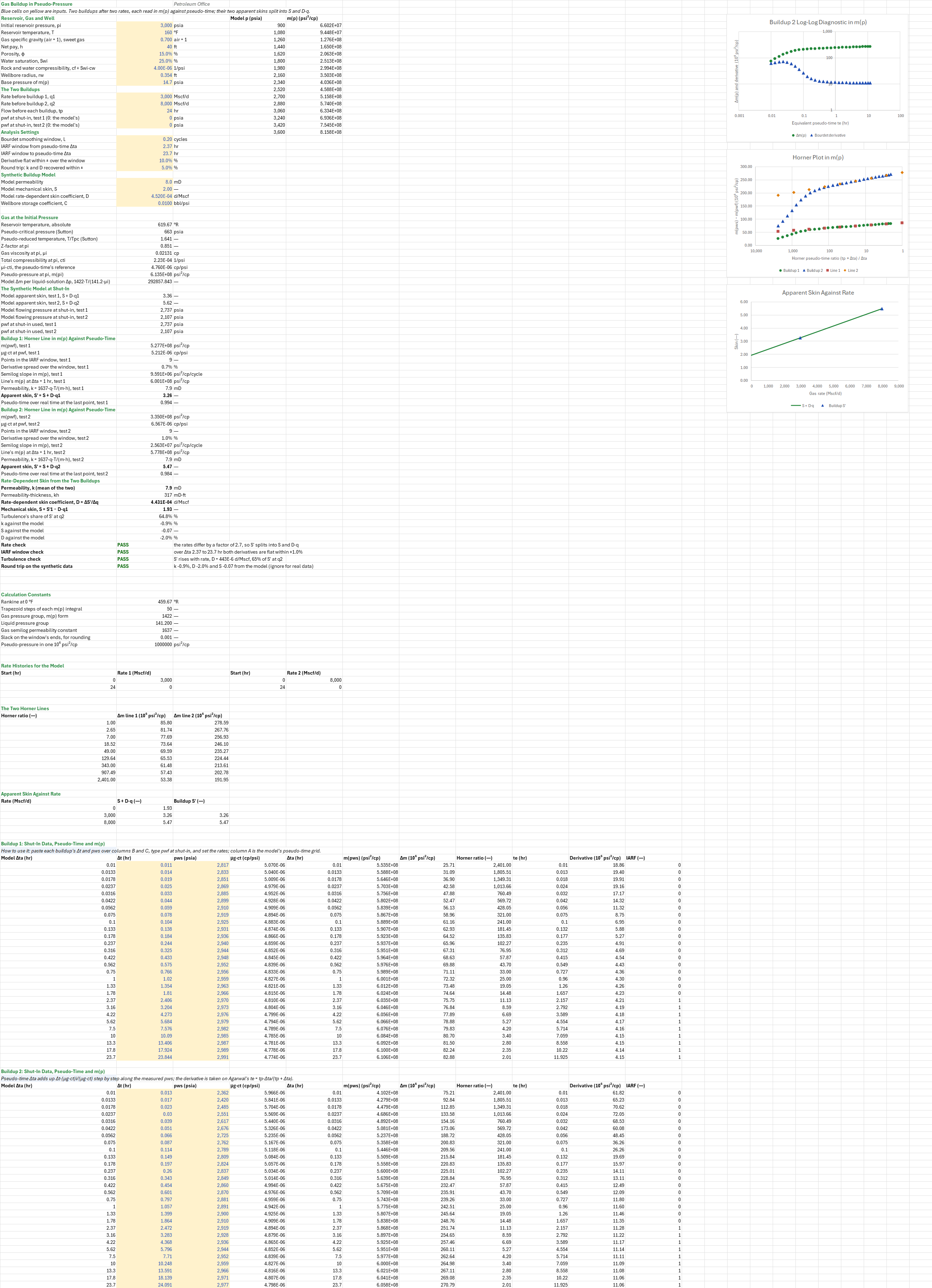
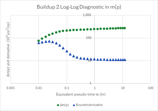
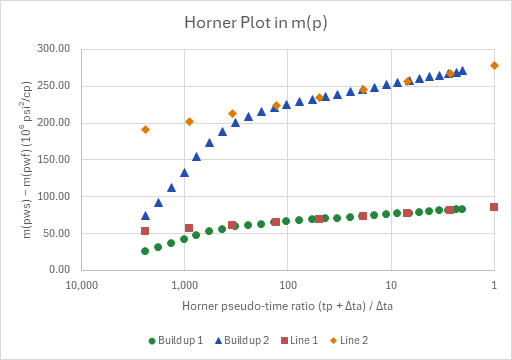
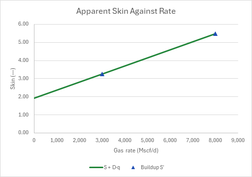
How to use it: Paste each buildup's Δt and pws over columns B and C. Type the flowing pressure at each shut-in into the two pwf inputs, set the rates and the flow time, and move the window onto the flat stretch of the derivative. Column A, the model's pseudo-time grid, is then unused, and the round-trip check doesn't apply. Two buildups after two different rates are needed for D. With only one, S′ is the result, and S = S′ − D·q needs a D from a correlation, such as the add-in's non-Darcy coefficient for a gas well. The sheet ships two synthetic buildups made from a model, so every result can be checked against the model that made it. A log-log plot draws the second buildup's Δm(p) and its derivative, a Horner plot draws both buildups with their lines, and a third plot draws S′ against rate.
Method: A gas well's skin grows with rate, S′ = S + D·q, because the flow near the well is turbulent; the two buildups' S′ therefore split into the mechanical skin S and the rate-dependent coefficient D. At pi the sheet takes Z by Dranchuk and Abou-Kassem at Sutton's pseudo-critical properties, and μg by Lee, Gonzalez and Eakin. It takes ct = (1 − Swi)·cg + cf with cg by its definition, and m(pi) from the pseudo-pressure integral (50 trapezoid steps). For each buildup row:
- μg·ct at pws, from the same functions;
- pseudo-time, Δta = Σ (μi·cti)·Δt/(μg·ct), the trapezoid of 1/(μg·ct) between rows, normalized at pi, from the flowing pressure at shut-in;
- m(pws) − m(pwf), the Horner ratio (tp + Δta)/Δta, Agarwal's te = tp·Δta/(tp + Δta), and the Bourdet derivative of Δm against ln te.
The Horner line is the least-squares line of m(pws) against log₁₀ of the ratio over the window's rows. Its slope's magnitude is m, and its value at Δta = 1 hr is m1hr. Then k = 1637·q·T/(m·h), and S′ = 1.151·[(m1hr − m(pwf))/m − log₁₀(k/(φ·μi·cti·rw²)) + 3.23], the liquid Horner skin with m(p) for p and μi·cti for μ·ct. D = (S′2 − S′1)/(q2 − q1), S = S′1 − D·q1, and k is the two buildups' mean.
- The synthetic buildups are the liquid solution written in m(p) and pseudo-time, which is what the two variables are for. The vertical-well model with storage and skin gives the buildup of a well with storage C and skin S + D·q, at q from 0 to tp and then shut in, on a grid of pseudo-times, with B = 1 and μi·cti in the diffusivity. Times 1422·T/(141.2·μi), that is Δm. A natural cubic spline through an m(p) table from 0.3·pi to 1.2·pi turns m(pws) back into pws. The real time Δt then follows by running the pseudo-time sum backwards along the model's pws. The analysis starts again from Δt and pws alone, as it would on a gauge's data.
Example: The gas and the well are the gas-inflow family's reference well: a 0.7 gravity sweet gas at 3,000 psia and 160 °F, 8 mD over 40 ft, rw 0.354 ft, a skin of 2, and D = 4.52 × 10⁻⁴ d/Mscf from the non-Darcy coefficient correlation with half the pay open. The sheet takes φ = 15 %, Swi = 25 %, cf = 4 × 10⁻⁶ 1/psi and C = 0.01 bbl/psi. At pi, Z = 0.8512, μi = 0.02131 cp, cti = 2.234 × 10⁻⁴ 1/psi and m(pi) = 6.135 × 10⁸ psi²/cp. The well flows 24 hr at 3,000 Mscf/d, and again at 8,000 Mscf/d, each to 2,737 and 2,107 psia, and each buildup is read for 23.7 hr of pseudo-time. Over the window from 2.37 to 23.7 hr, both derivatives are flat within ±1 %. Buildup 1 gives m = 9.591 × 10⁶ psi²/cp/cycle, k = 7.93 mD and S′ = 3.26. Buildup 2 gives m = 2.563 × 10⁷, k = 7.92 mD and S′ = 5.47. So k = 7.92 mD, D = 4.43 × 10⁻⁴ d/Mscf and S = 1.93. That is 0.9 % below the model's k, 2.0 % below its D and 0.07 below its skin, within the ±5 % tolerance. The small shortfall is the Horner line's, fitted over a buildup as long as the flow before it. Turbulence makes 65 % of S′ at 8,000 Mscf/d. Pseudo-time runs 0.6 % and 1.6 % behind real time at the end of the two buildups, more after the larger drawdown.
The sheet was checked against a standalone script. It rebuilds both buildups from the Engineering library's liquid PTA model and its Gauss-Legendre m(p), over the library's DAK, LGE and Sutton correlations, with m(p) inverted by bisection rather than a spline and cg by differencing DAK's Z. It then repeats the analysis with the library's Horner skin. It gives pwf 2,737.37 and 2,107.02 psia, slopes 9,590,592 and 25,629,117, k 7.93277 and 7.91599 mD, S′ 3.25768 and 5.47348, D 4.43159 × 10⁻⁴ and S 1.92821, all within 0.02 % of the sheet. Z and μg at pi are the gas-inflow sheets' (0.8512, 0.02131 cp), and the library's m(pi) is 613,556,320 psi²/cp, 0.007 % above the sheet's 50-step trapezoid. No printed two-rate gas buildup with pseudo-time and every input given was available, so the sheet is not compared with a published one.
Functions used
PO.PVT.Ppc.BySutton(SG_gas)
Calculates pseudo-critical pressure of hydrocarbon gas using Sutton (1985) correlation, [psi].
PO.PVT.Tpc.BySutton(SG_gas)
Calculates pseudo-critical temperature of hydrocarbon gas using Sutton (1985) correlation, [degR].
PO.PVT.Z.ByDAK(Ppr, Tpr)
Calculates gas compressibility factor (Z) using Dranchuk and Abou-Kassem (1975) equation of state, [dimensionless].
PO.PVT.Ug.ByLGE(Z, SG_gas, P, T_degR)
Calculates gas viscosity using Lee, Gonzales and Eakin (1966) correlation, [cP].
PO.PVT.Cg.ByDefinition(P, T_degR, SG_gas)
Calculates gas compressibility, [1/psi].
PO.Spline.Cubic.Interp(x_values, y_values, t)
Calculates interpolated value using natural cubic spline interpolation.
PO.PTA.Pw.VW(time, prod_data, B, Ul, C, Rw, S, Ct, porosity, h, K)
Calculates wellbore pressure drop for vertical well in infinite homogeneous reservoir, [psi].
PO.PTA.Horner.S(P1hr, Pwf, m, K, porosity, Ul, Ct, Rw)
Calculates the skin factor from the semilog straight line and abs(m); for a drawdown pass Pi as P1hr and the line's 1-hour pressure as Pwf, [dimensionless].
PO.DCA.Diag.Bourdet.SemiLog(x_values, y_values, t, L)
Calculates the classical Bourdet derivative dy/d(ln x) at point t, the log-domain estimator used for semilog and log-log well-test analysis. Multiply by LN(10) for a slope per log cycle.
Names (93)
| Name | Refers to | Comment |
|---|---|---|
PO.PVT.PseudoPLAMBDA |
=LAMBDA(p, t_r, sg_g, p_base, steps, IF((p<p_base)+(t_r<=0)+(sg_g<=0)+(steps<1)+(p_base/PO.PVT.Ppc.BySutton(sg_g)<0.01), NA(), LET(ppc, PO.PVT.Ppc.BySutton(sg_g), tpr, t_r/PO.PVT.Tpc.BySutton(sg_g), n, INT(steps), dp, (p-p_base)/n, f, MAP(p_base+dp*SEQUENCE(n+1, 1, 0), LAMBDA(x, LET(z, PO.PVT.Z.ByDAK(x/ppc, tpr), x/(PO.PVT.Ug.ByLGE(z, sg_g, x, t_r)*z)))), 2*dp*(SUM(f)-(INDEX(f, 1)+INDEX(f, n+1))/2)))) |
Real-gas pseudo-pressure m(p) = 2*integral of p/(ug*Z) dp from p_base to p (psi2/cp), trapezoid rule in steps; Z by DAK and ug by LGE at Sutton pseudo-criticals. p, p_base psia (p_base >= 7), t_r degR, sg_g air = 1. |
GPB_Pi |
$B$4 |
Initial reservoir pressure, pi, psia |
GPB_T |
$B$5 |
Reservoir temperature, T, °F |
GPB_SG |
$B$6 |
Gas specific gravity (air = 1), sweet gas, air = 1 |
GPB_h |
$B$7 |
Net pay, h, ft |
GPB_phi |
$B$8 |
Porosity, φ, % |
GPB_Swi |
$B$9 |
Water saturation, Swi, % |
GPB_cf |
$B$10 |
Rock and water compressibility, cf + Swi·cw, 1/psi |
GPB_rw |
$B$11 |
Wellbore radius, rw, ft |
GPB_Pbase |
$B$12 |
Base pressure of m(p), psia |
GPB_q1 |
$B$14 |
Rate before buildup 1, q1, Mscf/d |
GPB_q2 |
$B$15 |
Rate before buildup 2, q2, Mscf/d |
GPB_tp |
$B$16 |
Flow before each buildup, tp, hr |
GPB_Pwf1 |
$B$17 |
pwf at shut-in, test 1 (0: the model's), psia |
GPB_Pwf2 |
$B$18 |
pwf at shut-in, test 2 (0: the model's), psia |
GPB_L |
$B$20 |
Bourdet smoothing window, L, cycles |
GPB_From |
$B$21 |
IARF window from pseudo-time Δta, hr |
GPB_To |
$B$22 |
IARF window to pseudo-time Δta, hr |
GPB_Flat |
$B$23 |
Derivative flat within ± over the window, % |
GPB_Tol |
$B$24 |
Round trip: k and D recovered within ±, % |
GPB_ModelK |
$B$26 |
Model permeability, mD |
GPB_ModelS |
$B$27 |
Model mechanical skin, S |
GPB_ModelD |
$B$28 |
Model rate-dependent skin coefficient, D, d/Mscf |
GPB_C |
$B$29 |
Wellbore storage coefficient, C, bbl/psi |
GPB_Inputs |
$B$4:$B$29 |
The reservoir, the gas and the well, the two rates and flow time, the shut-in pressures, the window and tolerances, and the synthetic model |
GPB_TR |
$B$32 |
Reservoir temperature, absolute, °R |
GPB_Ppc |
$B$33 |
Pseudo-critical pressure (Sutton), psia |
GPB_Tpr |
$B$34 |
Pseudo-reduced temperature, T/Tpc (Sutton) |
GPB_Zi |
$B$35 |
Z-factor at pi |
GPB_Mui |
$B$36 |
Gas viscosity at pi, μi, cp |
GPB_Cti |
$B$37 |
Total compressibility at pi, cti, 1/psi |
GPB_McI |
$B$38 |
μi·cti, the pseudo-time's reference, cp/psi |
GPB_mPi |
$B$39 |
Pseudo-pressure at pi, m(pi), psi²/cp |
GPB_Scale |
$B$40 |
Model Δm per liquid-solution Δp, 1422·T/(141.2·μi) |
GPB_S1 |
$B$42 |
Model apparent skin, test 1, S + D·q1 |
GPB_S2 |
$B$43 |
Model apparent skin, test 2, S + D·q2 |
GPB_PwfModel1 |
$B$44 |
Model flowing pressure at shut-in, test 1, psia |
GPB_PwfModel2 |
$B$45 |
Model flowing pressure at shut-in, test 2, psia |
GPB_PwfU1 |
$B$46 |
pwf at shut-in used, test 1, psia |
GPB_PwfU2 |
$B$47 |
pwf at shut-in used, test 2, psia |
GPB_mPwf1 |
$B$49 |
m(pwf), test 1, psi²/cp |
GPB_McPwf1 |
$B$50 |
μg·ct at pwf, test 1, cp/psi |
GPB_N1 |
$B$51 |
Points in the IARF window, test 1 |
GPB_Flat1 |
$B$52 |
Derivative spread over the window, test 1, % |
GPB_M1 |
$B$53 |
Semilog slope in m(p), test 1, psi²/cp/cycle |
GPB_m1hr1 |
$B$54 |
Line's m(p) at Δta = 1 hr, test 1, psi²/cp |
GPB_k1 |
$B$55 |
Permeability, k = 1637·q·T/(m·h), test 1, mD |
GPB_Sa1 |
$B$56 |
Apparent skin, S′ = S + D·q1 |
GPB_TaRatio1 |
$B$57 |
Pseudo-time over real time at the last point, test 1 |
GPB_mPwf2 |
$B$59 |
m(pwf), test 2, psi²/cp |
GPB_McPwf2 |
$B$60 |
μg·ct at pwf, test 2, cp/psi |
GPB_N2 |
$B$61 |
Points in the IARF window, test 2 |
GPB_Flat2 |
$B$62 |
Derivative spread over the window, test 2, % |
GPB_M2 |
$B$63 |
Semilog slope in m(p), test 2, psi²/cp/cycle |
GPB_m1hr2 |
$B$64 |
Line's m(p) at Δta = 1 hr, test 2, psi²/cp |
GPB_k2 |
$B$65 |
Permeability, k = 1637·q·T/(m·h), test 2, mD |
GPB_Sa2 |
$B$66 |
Apparent skin, S′ = S + D·q2 |
GPB_TaRatio2 |
$B$67 |
Pseudo-time over real time at the last point, test 2 |
GPB_k |
$B$69 |
Permeability, k (mean of the two), mD |
GPB_kh |
$B$70 |
Permeability-thickness, kh, mD·ft |
GPB_D |
$B$71 |
Rate-dependent skin coefficient, D = ΔS′/Δq, d/Mscf |
GPB_S |
$B$72 |
Mechanical skin, S = S′1 − D·q1 |
GPB_TurbShare |
$B$73 |
Turbulence's share of S′ at q2, % |
GPB_kErr |
$B$74 |
k against the model, % |
GPB_SErr |
$B$75 |
S against the model |
GPB_DErr |
$B$76 |
D against the model, % |
GPB_RateCheck |
$B$77 |
Rate check verdict |
GPB_RateCheckNote |
$C$77 |
Rate check comment |
GPB_WindowCheck |
$B$78 |
IARF window check verdict |
GPB_WindowCheckNote |
$C$78 |
IARF window check comment |
GPB_TurbCheck |
$B$79 |
Turbulence check verdict |
GPB_TurbCheckNote |
$C$79 |
Turbulence check comment |
GPB_TripCheck |
$B$80 |
Round trip on the synthetic data verdict |
GPB_TripCheckNote |
$C$80 |
Round trip on the synthetic data comment |
GPB_Results |
$B$32:$B$80 |
The gas at pi, the model at shut-in, each buildup's Horner line, k and S′, the mean k, D and S, the round trip and the checks |
GPB_R0 |
$B$85 |
Rankine at 0 °F, °R |
GPB_Steps |
$B$86 |
Trapezoid steps of each m(p) integral |
GPB_K1422 |
$B$87 |
Gas pressure group, m(p) form |
GPB_K1412 |
$B$88 |
Liquid pressure group |
GPB_K1637 |
$B$89 |
Gas semilog permeability constant |
GPB_Mega |
$B$91 |
Pseudo-pressure in one 10⁶ psi²/cp, psi²/cp |
GPB_Eps |
$B$90 |
Slack on the window's ends, for rounding |
GPB_MpTable |
$D$4:$E$19 |
Pressures from 0.3·pi to 1.2·pi and their m(p), which the model's spline reads backwards |
GPB_PTab |
$D$4:$D$19 |
The m(p) table's pressures, psia |
GPB_MTab |
$E$4:$E$19 |
The m(p) table's pseudo-pressures, psi²/cp |
GPB_Rates1 |
$A$96:$B$97 |
Test 1's model: q1 from 0 to tp, then shut in |
GPB_Rates2 |
$D$96:$E$97 |
Test 2's model: q2 from 0 to tp, then shut in |
GPB_Lines |
$A$102:$C$110 |
Each buildup's Horner line as Δm(p), from a ratio of 1 to the data's largest |
GPB_Curve |
$A$114:$C$116 |
The line S + D·q from q = 0, and the two buildups' apparent skins on it |
GPB_Data1 |
$A$122:$C$149 |
Buildup 1: the model's pseudo-time grid, and Δt and pws (the model's until you paste a gauge's) |
GPB_Analysis1 |
$D$122:$K$149 |
Buildup 1 per row: μg·ct at pws, pseudo-time, m(pws), Δm, the Horner ratio, te, the Bourdet derivative and the IARF window |
GPB_Data2 |
$A$154:$C$181 |
Buildup 2: the model's pseudo-time grid, and Δt and pws (the model's until you paste a gauge's) |
GPB_Analysis2 |
$D$154:$K$181 |
Buildup 2 per row: μg·ct at pws, pseudo-time, m(pws), Δm, the Horner ratio, te, the Bourdet derivative and the IARF window |
Details
| Inserts | 181 rows × 11 columns |
| Category | Pressure Transient Analysis |
| For agents and tools | Descriptor (.md) |