Gas Water-Drive Diagnostic (Cole Plot)
Description
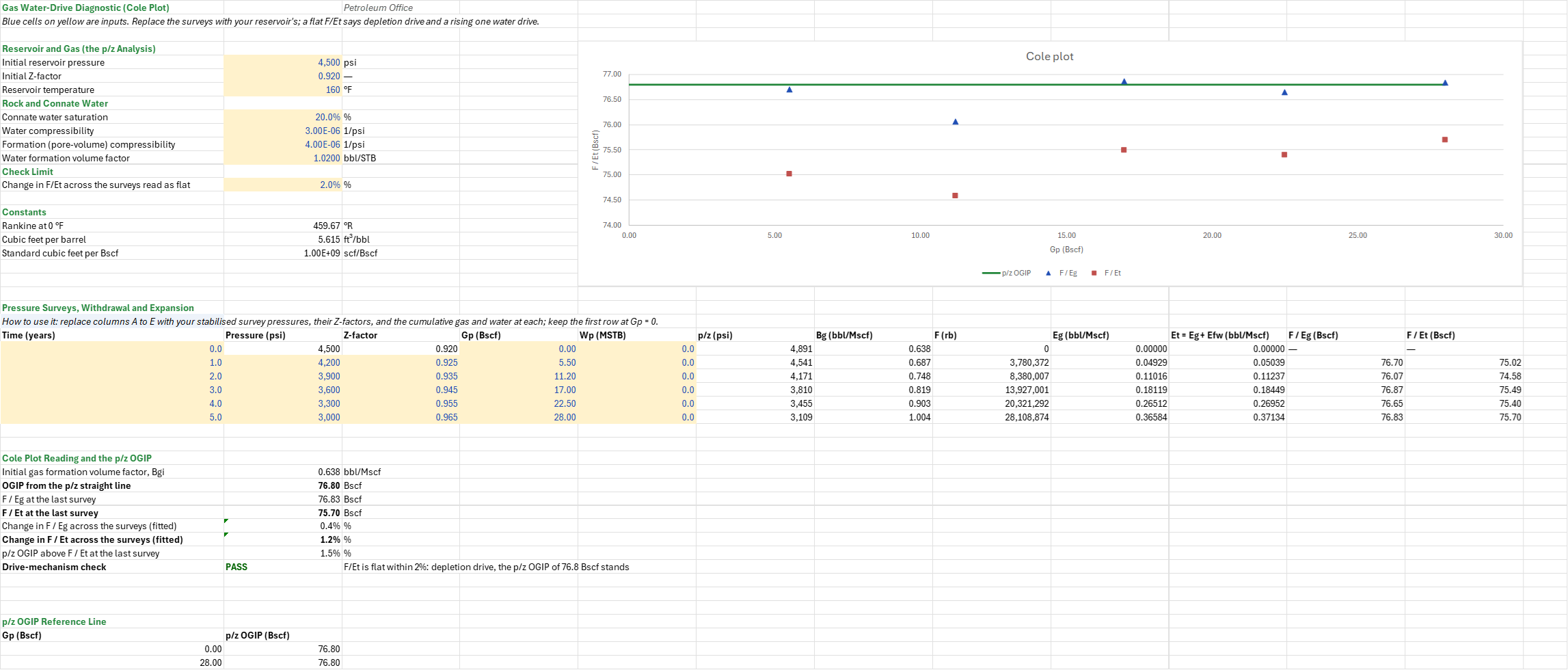
Is a gas reservoir depleting on its own, or is an aquifer pushing water in, and can its p/z straight line be trusted? You enter the initial pressure, Z-factor and temperature, the connate water saturation, the water and pore-volume compressibilities and Bw, and the pressure surveys with their Z-factors and cumulative gas and water. You read off the Cole plot of F/Eg and F/Et against cumulative gas, the trend of F/Et across the surveys with a drive check, and how far the p/z gas in place sits above the Cole value.
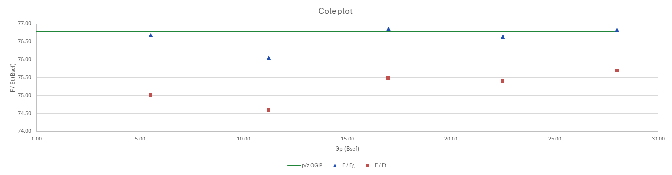
The p/z plot itself hides a water drive: a moderate one bends the line so gently that it looks straight and overstates the gas in place. The Cole plot shows it. The sheet computes, at each pressure survey, the underground withdrawal F, the gas expansion Eg and Et, Eg plus the rock and connate-water expansion, and plots F/Eg and F/Et against the cumulative gas. With no aquifer, F/Et equals the gas in place at every survey and the points lie on a horizontal line. Water influx adds to F without adding to Et, so the points climb. They fall when the reservoir is overpressured or its rock compressibility is understated.
The sheet reads the trend as the change in F/Et across the surveys, from the least-squares slope against Gp, and a check compares it with a limit. Beside it are the OGIP of the p/z straight line, F/Eg and F/Et at the last survey, and how far the p/z OGIP sits above the Cole value. The Cole plot draws F/Eg and F/Et against Gp, with the p/z OGIP as a horizontal reference.
Parameters:
- Reservoir and gas: the initial pressure
COLE_Pi(psi), its Z-factorCOLE_Ziand the reservoir temperatureCOLE_T(°F) - Rock and connate water: the connate water saturation
COLE_Swi, the water and pore-volume compressibilitiesCOLE_cwandCOLE_cf(1/psi), and BwCOLE_Bw(bbl/STB) for the produced water - Check limit: the change in F/Et across the surveys read as flat,
COLE_TrendMax - Surveys: time, pressure, Z-factor, cumulative gas Gp (Bscf) and cumulative water Wp (MSTB), the region
COLE_Surveys. The first row is the initial survey at Gp = 0, from the initial conditions.
How to use it: Replace the survey rows with stabilised static pressures, the Z-factor of the gas at each pressure and reservoir temperature, and the cumulative gas and water at each survey date. Produced water counts in F, so a reservoir that makes water must have it entered. The early surveys carry the most error, because Eg is small after a small pressure drop: a 1 % error in the initial pressure moves the first survey's F/Et by more than 10 %. Read the trend from the later surveys, and check Pi before calling a water drive.
Method: For a gas reservoir the material balance is F = G·Et + We·Bw, with F = Gp·Bg + Wp·Bw, Eg = Bg − Bgi and Et = Eg + Efw, where Efw = Bgi·(cw·Swi + cf)/(1 − Swi)·(pi − p), the rock and connate-water expansion with no gas cap. Dividing by Et gives F/Et = G + We·Bw/Et: flat at G with no influx. Bg comes from its definition at each survey's pressure, Z and temperature. Each survey's F/Eg equals the single-survey OGIP of the p/z analysis, Gp/(1 − (p/z)/(pi/zi)). The trend is the least-squares slope of F/Et against Gp over the surveys, times their Gp span, over their mean F/Et. The p/z OGIP is the least-squares p/z regression over every survey, the initial one included. The drive check fails when the trend rises past the limit, warns when it falls past it, and passes otherwise.
Example: The surveys are the Gas Reservoir p/z Analysis sheet's: 4,500 psi (Z 0.92) at Gp = 0, then five annual surveys down to 3,000 psi (Z 0.965) at 28 Bscf, with no water produced. The temperature is the Gas Reservoir Production Forecast sheet's 160 °F, and the rock and water are the Aquifer Model Matching sheet's: Swi 20 %, cw 3 × 10⁻⁶ and cf 4 × 10⁻⁶ 1/psi, Bw 1.02. F/Eg runs 76.70, 76.07, 76.87, 76.65 and 76.83 Bscf, the single-survey OGIPs of the p/z sheet, and the p/z line gives 76.80 Bscf. With the rock and water, F/Et runs 75.02, 74.58, 75.49, 75.40 and 75.70 Bscf, a change of 1.2 % across the surveys, flat within 2 %: depletion drive. The p/z OGIP sits 1.5 % above F/Et at the last survey, the share of the withdrawal the rock and water supplied. Overstating Pi by 50 psi makes F/Et climb 11.6 %, and the check fails it as a water drive; understating it by 50 psi makes F/Et fall 11.8 %, and the check warns. Leaving the rock and water out gives F/Et = F/Eg, with a change of 0.4 %.
Functions used
PO.MBE.Gas.Pz(P, z)
Calculates p/z ratio for gas material balance analysis, [psi].
PO.PVT.Bg.ByDefinition(P, T_degR, Z)
Calculates gas formation volume factor, [rcf/scf].
PO.MBE.F.Gas(Gp, Bg, Wp, Bw)
Calculates underground withdrawal for gas reservoir, [bbl]. F = Gp*Bg + Wp*Bw.
PO.MBE.Exp.Eg.Gas(Bg, Bgi)
Calculates gas expansion for pure gas reservoirs, [RB/scf]. Eg = Bg - Bgi.
PO.MBE.Exp.Efw(Boi, cw, cf, Swc, m, deltaP)
Calculates formation/water expansion term (Efw), [bbl/STB]. Accounts for rock compaction and connate water expansion.
PO.MBE.Gas.OGIP.Reg(P, z, Gp)
Estimates original gas in place from a least-squares straight line through p/z against Gp, extrapolated to p/z = 0, in the unit of Gp, [scf].
Names (24)
| Name | Refers to | Comment |
|---|---|---|
COLE_Pi |
$B$5 |
Initial reservoir pressure, psi |
COLE_Zi |
$B$6 |
Initial Z-factor |
COLE_T |
$B$7 |
Reservoir temperature, °F |
COLE_Swi |
$B$9 |
Connate water saturation, % |
COLE_cw |
$B$10 |
Water compressibility, 1/psi |
COLE_cf |
$B$11 |
Formation (pore-volume) compressibility, 1/psi |
COLE_Bw |
$B$12 |
Water formation volume factor, bbl/STB |
COLE_TrendMax |
$B$14 |
Change in F/Et across the surveys read as flat, % |
COLE_Inputs |
$B$5:$B$14 |
Initial pressure, Z and temperature, the rock and connate water, and the flatness limit |
COLE_R0 |
$B$17 |
Rankine at 0 °F, °R |
COLE_CfPerBbl |
$B$18 |
Cubic feet per barrel, ft³/bbl |
COLE_ScfPerBscf |
$B$19 |
Standard cubic feet per Bscf, scf/Bscf |
COLE_Surveys |
$A$26:$E$31 |
Pressure surveys: time, pressure, Z-factor, cumulative gas and cumulative water |
COLE_Cole |
$D$27:$L$31 |
Each survey's Gp, F, Eg, Et and the Cole ratios F/Eg and F/Et |
COLE_Bgi |
$B$35 |
Initial gas formation volume factor, Bgi, bbl/Mscf |
COLE_OgipPz |
$B$36 |
OGIP from the p/z straight line, Bscf |
COLE_FEg |
$B$37 |
F / Eg at the last survey, Bscf |
COLE_FEt |
$B$38 |
F / Et at the last survey, Bscf |
COLE_TrendEg |
$B$39 |
Change in F / Eg across the surveys (fitted), % |
COLE_Trend |
$B$40 |
Change in F / Et across the surveys (fitted), % |
COLE_Excess |
$B$41 |
p/z OGIP above F / Et at the last survey, % |
COLE_DriveCheck |
$B$42 |
Drive-mechanism check verdict |
COLE_DriveCheckNote |
$C$42 |
Drive-mechanism check comment |
COLE_Results |
$B$35:$B$42 |
Bgi, the p/z OGIP, the last survey's F/Eg and F/Et, their trends, the p/z excess and the drive check |
Details
| Inserts | 49 rows × 12 columns |
| Category | Material Balance Equation |
| For agents and tools | Descriptor (.md) |